
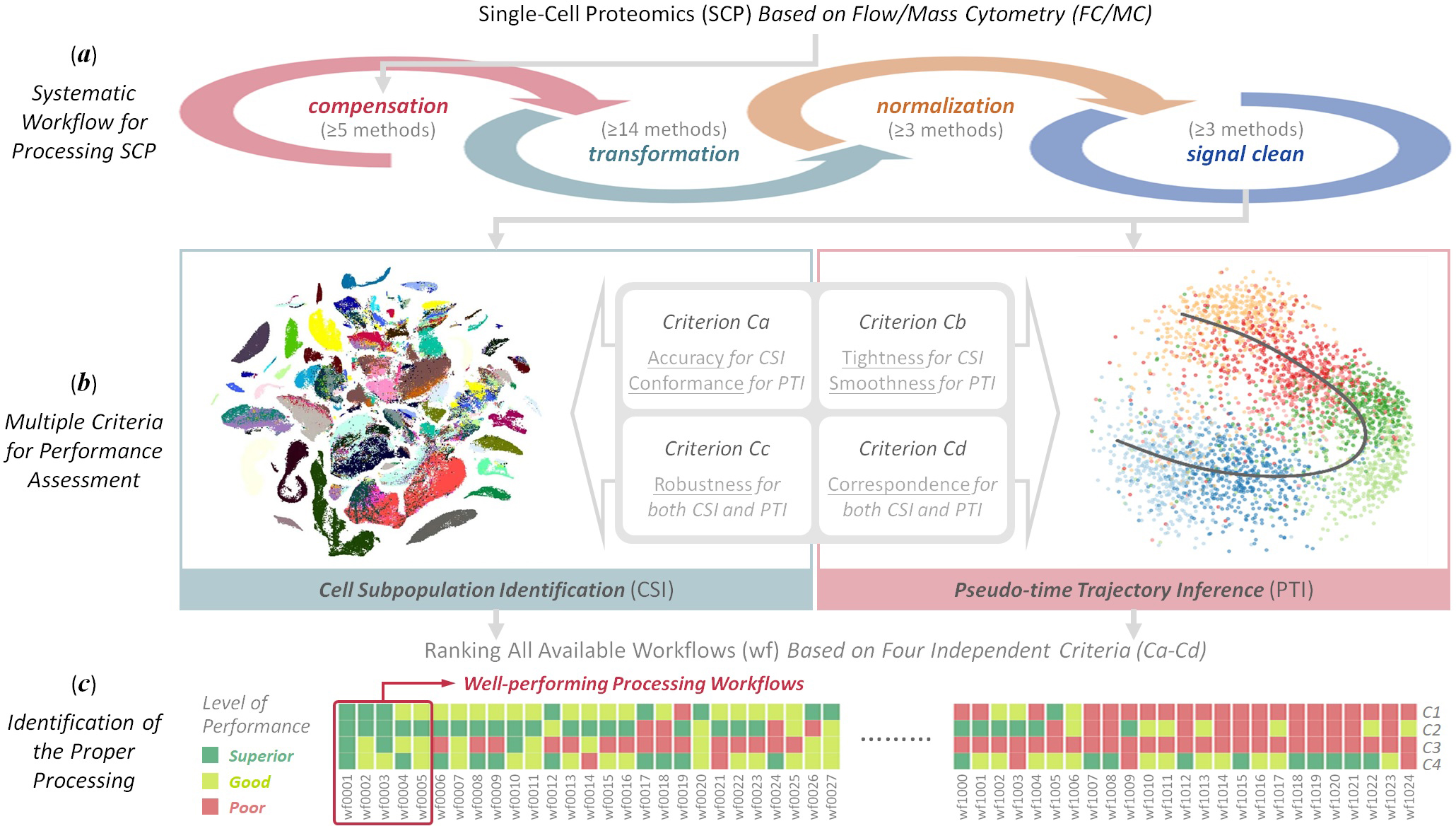
ANPELA is designed for navigating the data processing for cytometry-based Single-Cell Proteomics (SCP).
Desktop Software of ANPELA is downloadable at Download. R Package of ANPELA is availale at https://github.com/idrblab/ANPELA.
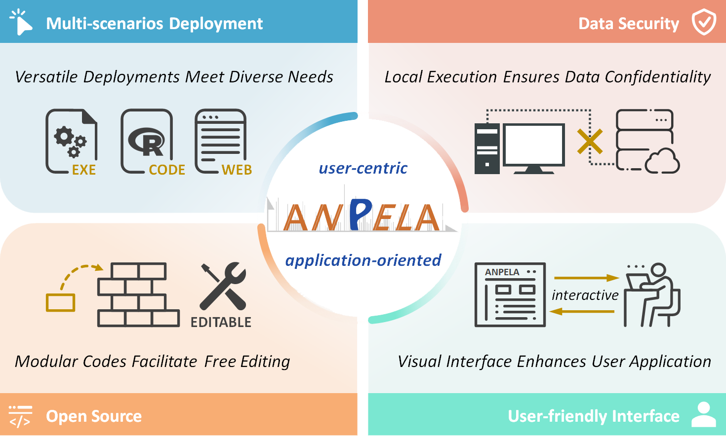
ANPELA 3.0 has significantly improved its practicality, focusing primarily on the following points: 1. multi-scenarios deployment (versatile choices meet diverse user needs, as shown in 'Multi-scenarios Deployments of ANPELA'); 2. data security (local execution ensures data confidentiality); 3. open source (modular codes facilitate readers’ free editing); and 4. user-friendly interface (the visual interface enhances user application).
Citing the ANPELA:
1. HC Sun, Y Zhou, RY Jiang,..., F Zhu*. Navigating the data processing for cytometry-based single-cell proteomics. Nature Protocols. doi:10.1038/s41596-025-01257-2, 2025
Four Key Characteristics of ANPELA:
Multi-scenarios Deployment (versatile choices meet diverse user needs); Data Security (local execution ensures data confidentiality); Open Source (modular codes facilitate users’ free editing); and User-friendly Interface (visual interface enhances user application).
Browser and Operating System (OS) Tested for Smoothly Running ANPELA:
ANPELA is powered by R shiny. It is free and open to all users with no login requirement and can be readily accessed by a variety of popular web browsers and operating systems as shown below.
| OS | Chrome | Firefox | Edge | Safari |
|---|---|---|---|---|
| Linux (Ubuntu-17.04) | v78.0.3904.108 | v52.0.1 | n/a | n/a |
| MacOS (v10.1) | v78 | v71 | n/a | v8 |
| Windows (v10) | v78.0.3904.108 | v70.0.1 | v44.18362.449.0 | n/a |
Multi-scenarios Deployments of ANPELA:
| Use Form | Access Method | Usage Instructions | Target Audience |
|---|---|---|---|
| Desktop Software | Download | Software's "Textual Tutorial" and "Interactive Tutorial" | Users who want to traverse all processing workflows and select the optimal workflow; Users with no background in R programming |
| Web Platform | https://idrblab.org/anpela2025/ | Website's "Textual Tutorial" and "Interactive Tutorial" | Users who need only a specific data processing workflow |
| R Package | GitHub | idrblab/ANPELA | Users who want to traverse all processing workflows and select the optimal workflow; Users with a background in R programming |
ANPELA 2.0 is capable of AUTOMATICALLY detecting the raw SCP flow-cytometry-standard file (.fcs) generated by flow/mass-cytometry. ANPELA 1.0 can detect the diverse formats of data generated by all quantification software for SWATH-MS, Peak Intensity and Spectral Counting.
The Previous Version of ANPELA can be accessed at: http://idrblab.cn/anpela2020/
Thanks a million for using and improving ANPELA, and please feel free to report any errors to Dr. Sun.
Welcome to Download the Sample Data for Testing and for File Format Correcting
- Cell Subpopulation Identification
The compressed file (in the .zip format) containing raw FCS files generated by flow cytometry, and the corresponding data of golden standards for performance assessment using Criterion Cd could be downloaded .
The compressed file (in the .zip format) containing raw FCS files generated by mass cytometry, and the corresponding data of golden standards for performance assessment using Criterion Cd could be downloaded .
- Pseudo-time Trajectory Inference
The compressed file (in the .zip format) containing raw FCS files generated by flow cytometry, the metadata file providing the correspondence between filenames and time points, as well as the corresponding data of pathway hierarchy for performance assessment using Criterion Cd could be downloaded .
The compressed file (in the .zip format) containing raw FCS files generated by mass cytometry, the metadata file providing the correspondence between filenames and time points, as well as the corresponding data of pathway hierarchy for performance assessment using Criterion Cd could be downloaded .
Summary and Visualization of the Uploaded Raw SCP Data
- The Expression of Proteins (columns) in Different Cells (rows)

- Stacked Density Plot for Different Samples
WARNING
The filenames of your uploaded FCS files are inconsistent with those of your uploaded metadata file.
Note that ANPELA requires the user to upload FCS files whose filename order is exactly the same as that of the metadata file.
Please refresh the page and reupload the raw FCS files & metadata in the correct format.
WARNING
The number of uploaded FCS file(s) is not enough for the subsequent analysis.
Particularly, for two-class research, at least two samples for each class are required; for trajectory inference research, at least two time points are required.
Please refresh the page and reupload the raw FCS files & metadata in the correct format.
Summary and Visualization of the Uploaded Raw SCP Data
- The Expression of Proteins (columns) in Different Cells (rows)
- Stacked Density Plot for Different Samples
WARNING
The filenames of your uploaded FCS files are inconsistent with those of your uploaded metadata file.
Note that ANPELA requires the user to upload FCS files whose filename order is exactly the same as that of the metadata file.
Please refresh the page and reupload the raw FCS files & metadata in the correct format.
WARNING
The number of uploaded FCS file(s) is not enough for the subsequent analysis.
Particularly, for two-class research, at least two samples for each class are required; for trajectory inference research, at least two time points are required.
Please refresh the page and reupload the raw FCS files & metadata in the correct format.
Summary and Visualization of the Uploaded Raw Data
The Data File is Successfully Uploaded, which is Recognized as the Resulting Data File Generated by the Quantification Software:
Please Upload the Corresponding Label File Indicating the Classes of Each Sample
Summary and Visualization of the Uploaded Raw Data
The Data File is Successfully Uploaded, which is Recognized as the Resulting Data File Generated by the Quantification Software:
Please Upload the Corresponding Label File Indicating the Classes of Each Sample
Summary and Visualization of the Uploaded Raw Data
The Data File is Successfully Uploaded, which is Recognized as the Resulting Data File Generated by the Quantification Software:
Please Upload the Corresponding Label File Indicating the Classes of Each Sample
Summary and Visualization of the Uploaded Raw Data
The Label File is Successfully Uploaded, Please Upload the Corresponding Data File Generated by Popular Software of the Selected MOA
Summary and Visualization of the Uploaded Raw Data
The Label File is Successfully Uploaded, Please Upload the Corresponding Data File Generated by Popular Software of the Selected MOA
Summary and Visualization of the Uploaded Raw Data
The Label File is Successfully Uploaded, Please Upload the Corresponding Data File Generated by Popular Software of the Selected MOA
Instruction to the User
1. Please Choose a Format File Unified by ANPELA in the Left Side Panel
2. Please Process the Uploaded Data by Clicking the "Upload Data" Button in the Left Side Panel
Instruction to the User
1. Please Choose Your Preferred "Mode of Acquisition (MOA)" in the Left Side Panel
SWATH-MS Data (sequential windowed acquisition of all theoretical fragment ion mass spectra)
Sample data file of this MOA could be downloaded HERE, together with an additional label file
Peak Intensity (pre-processing the data acquired based on precursor ion signal intensity)
Sample data file of this MOA could be downloaded HERE, together with an additional label file
Spectral counting (pre-processing the data acquired based on MS2 spectral counting)
Sample data file of this MOA could be downloaded HERE, together with an additional label file
2. Please Upload the Data File Generated by Popular Software of the Selected MOA in the Left Side Panel
3. Please Upload the Label File Indicating the Classes of Each Sample in the Left Side Panel
4. Please Process the Uploaded Data by Clicking the "Upload Data" Button in the Left Side Panel
Summary and Visualization of Raw Data
A. Summary of the Raw Data
B. Distribution of Protein Intensities Before and After Log Transformation
Summary and Visualization of the Uploaded Raw Data
A. Summary of the Raw Data
B. Distribution of Protein Intensities Before and After Log Transformation
Summary and Visualization of the Uploaded Raw Data
A. Summary of the Raw Data
B. Distribution of Protein Intensities Before and After Log Transformation
Summary and Visualization of the Uploaded Raw Data
A. Summary of the Raw Data
B. Distribution of Protein Intensities Before and After Log Transformation
Summary and Visualization of the Uploaded Raw Data
A. Summary of the Raw Data
B. Distribution of Protein Intensities Before and After Log Transformation
Interactive Tutorial Launching:
The interactive tutorial is starting up, which usually takes a few to ten seconds.
If you encounter any issues, feel free to contact Dr. Sun at any time.