
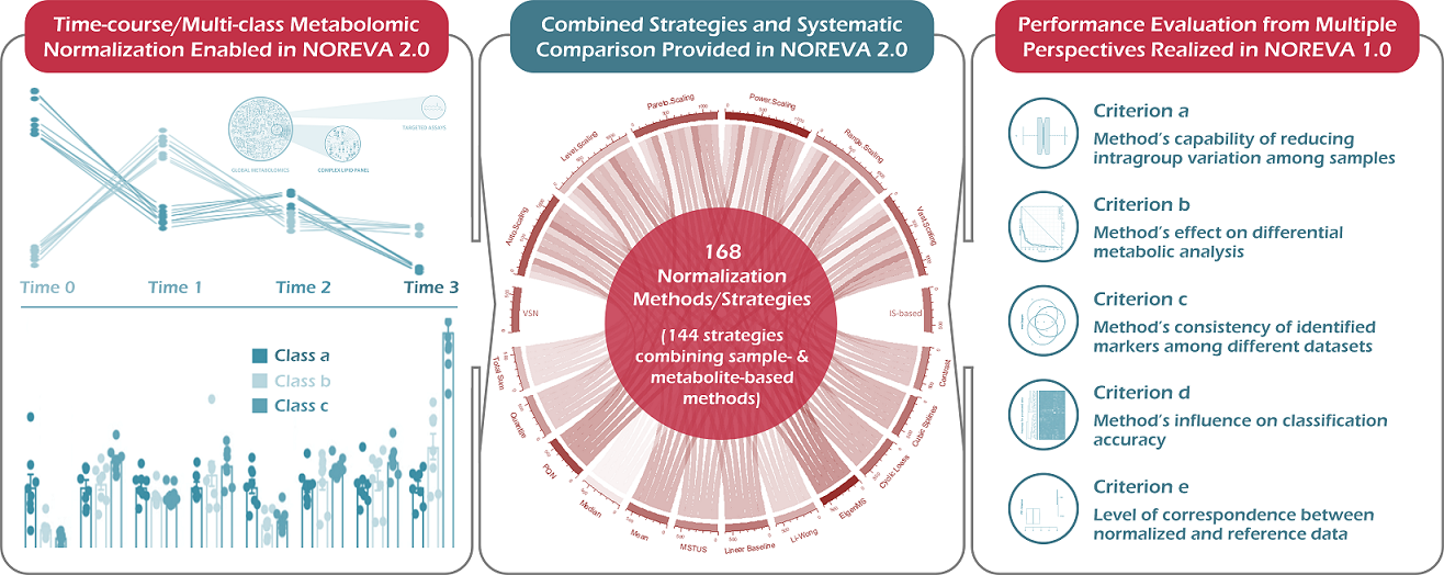
NOREVA 2.0 is constructed to enable the online services of (1) normalizing the time-course/multi-class metabolomic data using 168 methods/strategies, (2) evaluating the normalization performances from multiple perspectives, and (3) enabling the systematic comparison among all methods/strategies based on a comprehensive performance ranking. Particularly, five well-established criteria, each with a distinct underlying theory, are integrated to ensure a much more comprehensive evaluation than any single criterion. Besides its largest and most diverse sets of normalization methods/strategies among all available tools, NOREVA provided a unique feature of allowing the quality control-based correction sequentially followed by data normalization.
Citing the NOREVA:
1. J. B. Fu, Y. Zhang, Y. X. Wang, H. N. Zhang, J. Liu, J. Tang, Q. X. Yang, H. C. Sun, W. Q. Qiu, Y. H. Ma, Z. R. Li, M. Y. Zheng, F. Zhu*. Optimization of metabolomic data processing using NOREVA. Nature Protocols. 17(1): 129-151 (2022). doi: 10.1038/s41596-021-00636-9; PubMed ID: 34952956
2. Q. X. Yang, Y. X. Wang, Y. Zhang, F. C. Li, W. Q. Xia, Y. Zhou, Y. Q. Qiu, H. L. Li, F. Zhu*. NOREVA: enhanced normalization and evaluation of time-course and multi-class metabolomic data. Nucleic Acids Research. 48(W1): 436-448 (2020). doi: 10.1093/nar/gkaa258; PubMed ID: 32324219
Browser and Operating System (OS) Tested for Smoothly Running NOREVA:
NOREVA is powered by R shiny. It is free and open to all users with no login requirement and can be readily accessed by a variety of popular web browsers and operating systems as shown below.
The Previous Version of NOREVA can be accessed at: http://idrblab.cn/noreva2017/
Thanks a million for using and improving NOREVA, and please feel free to report any errors to Dr. YANG at yangqx@cqu.edu.cn.
Significantly Enhanced Function of NOREVA 2.0:
The function of NOREVA 2.0 is enhanced by: (1) realizing the normalization & evaluation of both time-course (J Biol Chem. 292: 19556-64, 2017) and multi-class (Science. 363: 644-9, 2019) metabolomic data, (2) adding the combined strategy of enhanced normalization performance that was frequently adopted in metabolomics (Nat Protoc. 6: 743-60, 2011; Brief Bioinform. pii: bbz137, 2019) and (3) allowing the systematic comparison among 168 normalization methods/strategies based on a comprehensive performance ranking. Due to the dramatically increased number of time-course/multi-class studies in recent years, NOREVA 2.0 is unique in assessing normalization for this emerging field, which further enhances its popularity in current metabolomics.
The Unique Function of NOREVA 1.0 (Nucleic Acids Res. 45: 162-70, 2017):
NOREVA enables the performance evaluation of various normalization methods from multiple perspectives, which integrates five well-established criteria (each with a distinct underlying theory) to ensure more comprehensive evaluation than any single criterion. (criterion a) Method’s capability of reducing intragroup variation among samples (J Proteome Res. 13: 3114-20, 2014); (criterion b) Method’s effect on differential metabolic analysis (Brief Bioinform. 19: 1-11, 2018); (criterion c) Method’s consistency of the identified metabolic markers among different datasets (Mol Biosyst. 11: 1235-40, 2015); (criterion d) Method’s influence on classification accuracy (Nat Biotechnol. 32: 896-902, 2014); (criterion e) Level of correspondence between the normalized and reference data (Brief Bioinform. 19: 1-11, 2018).
Summary and Visualization of the Uploaded Raw Metabolomic Data
- Summary of the Raw Data

- Visualization of Data Distribution
Welcome to Download the Sample Data for Testing and for File Format Correcting
- Time-course Metabolomic Study
Dataset with quality control samples (QCSs) could be downloaded and the corresponding data of golden standards for performance evaluation using Criterion e could be downloaded .
Dataset with internal standards (ISs) could be downloaded and the corresponding data of golden standards for performance evaluation using Criterion e could be downloaded .
Dataset without QCSs and ISs could be downloaded and the corresponding data of golden standards for performance evaluation using Criterion e could be downloaded .
- Multi-class Metabolomic Study
Dataset with quality control samples (QCSs) could be downloaded and the corresponding data of golden standards for performance evaluation using Criterion e could be downloaded .
Dataset with internal standards (ISs) could be downloaded and the corresponding data of golden standards for performance evaluation using Criterion e could be downloaded .
Dataset without QCSs and ISs could be downloaded and the corresponding data of golden standards for performance evaluation using Criterion e could be downloaded .
Summary and Visualization of the Uploaded Raw Metabolomic Data
- Summary of the Raw Data
- Visualization of Data Distribution
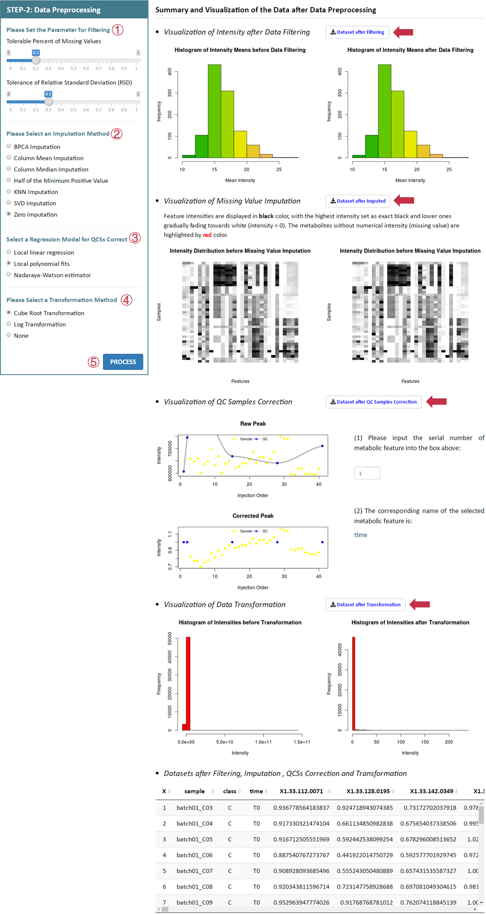
Introduction to the Data Preprocessing Step of NOREVA
- Data Filtering and Parameter Setting
Metabolomic data are filtered when the percent of missing values of each metabolite is larger than the tolerable cutoff. This cutoff is set by users with a default value of 0.2 (Chen J, et al. Anal Chem. 89: 5342-8, 2017). The RSD is the absolute measurement of batch-to-batch variation and a lower RSD indicates better reproducibility of the feature (Dunn WB, et al. Nat Protoc. 6: 1060-83, 2011). A metabolite will be deleted if its RSD across all quality controls (QCs) is higher than the threshold defined by users (the default is set to 0.3).
- Methods for Missing Value Imputation
There are seven methods provided here for missing value imputation. (1) BPCA Imputation imputes missing data with the values obtained from Bayesian principal component analysis regression (Oba S, et al. Bioinformatics. 19: 2088-96, 2003), and the number of principal components used for calculation should be set by users with a default value of 3. (2) Column Mean Imputation imputes missing values with the mean value of non-missing values in the corresponding metabolite (Huan T, et al. Anal Chem. 87: 1306-13, 2015). (3) Column Median Imputation imputes missing values with the median value of non-missing values in the corresponding metabolite (Huan T, et al. Anal Chem. 87: 1306-13, 2015). (4) Half of the Minimum Positive Value imputes missing values using the half of the minimum positive value in all metabolomics data (Taylor SL, et al. Brief Bioinform. 18: 312-20, 2017). (5) KNN Imputation aims to find K metabolites of interest which are similar to the metabolites with missing value, and the detail algorithm together with the corresponding parameters are provided in Tang J, et al. Brief Bioinform. doi: 10.1093/bib/bby127, 2019. (6) SVD Imputation analyzes the principle components that represent the entire matrix information and then to estimate the missing values by regressing against the principle components (Gan X, et al. Nucleic Acids Res. 34: 1608-19, 2006). (7) Zero Imputation replaces all missing values with zero (Gromski PS, et al. Metabolites. 4: 433-52, 2014).
- Methods for Data Transformation
There are two methods provided here for data transformation. (1) Cube Root Transformation is employed to improve the normality distribution of simple count data (Ho EN, et al. Drug Test Anal. 7: 414-9, 2015). (2) Log Transformation is a nonlinear conversion of data to decrease heteroscedasticity and obtain a more symmetric distribution prior to statistical analysis (Purohit PV, et al. OMICS. 8: 118-30, 2004). No transformation is allowed for data preprocessing by selecting the “None” option.
- QC Sample Correction and Parameter Setting of Regression Model
The correction strategy based on multiple QC samples is popular in evaluating the signal drifts and other systematic noise using mathematical algorithms (Luan H, et al. Anal Chim Acta. 1036: 66-72, 2018). The regression model for QC-RLSC including Nadaraya-Watson Estimator, Local Linear Regression and Local Polynomial Fits, which should be selected by users.
Summary and Visualization of the Data after Data Preprocessing
- Visualization of Intensity after Data Filtering
- Visualization of Missing Value Imputation
- Visualization of QC Samples Correction
Please input the serial number of metabolic feature
- Datasets after Filtering, Imputation , QCSs Correction and Transformation
Summary and Visualization of the Data after Data Preprocessing
- Visualization of Intensity after Data Filtering
- Visualization of Missing Value Imputation
- Visualization of Data Transformation
- Datasets after Filtering, Imputation and Transformation
Summary and Visualization of the Data after Data Preprocessing
- Visualization of Intensity after Data Filtering
- Visualization of Missing Value Imputation
- Visualization of Data Transformation
- Datasets after Filtering, Imputation and Transformation
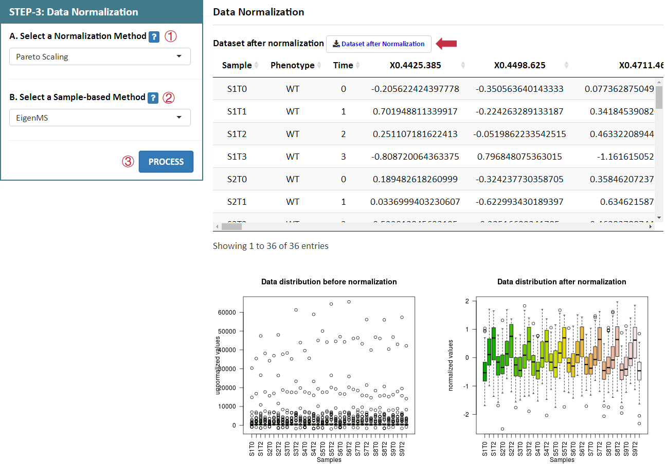
Introduction to the Data Normalization Step of NOREVA
- Normalization Strategy of Combining Sample-based and Metabolite-based Method
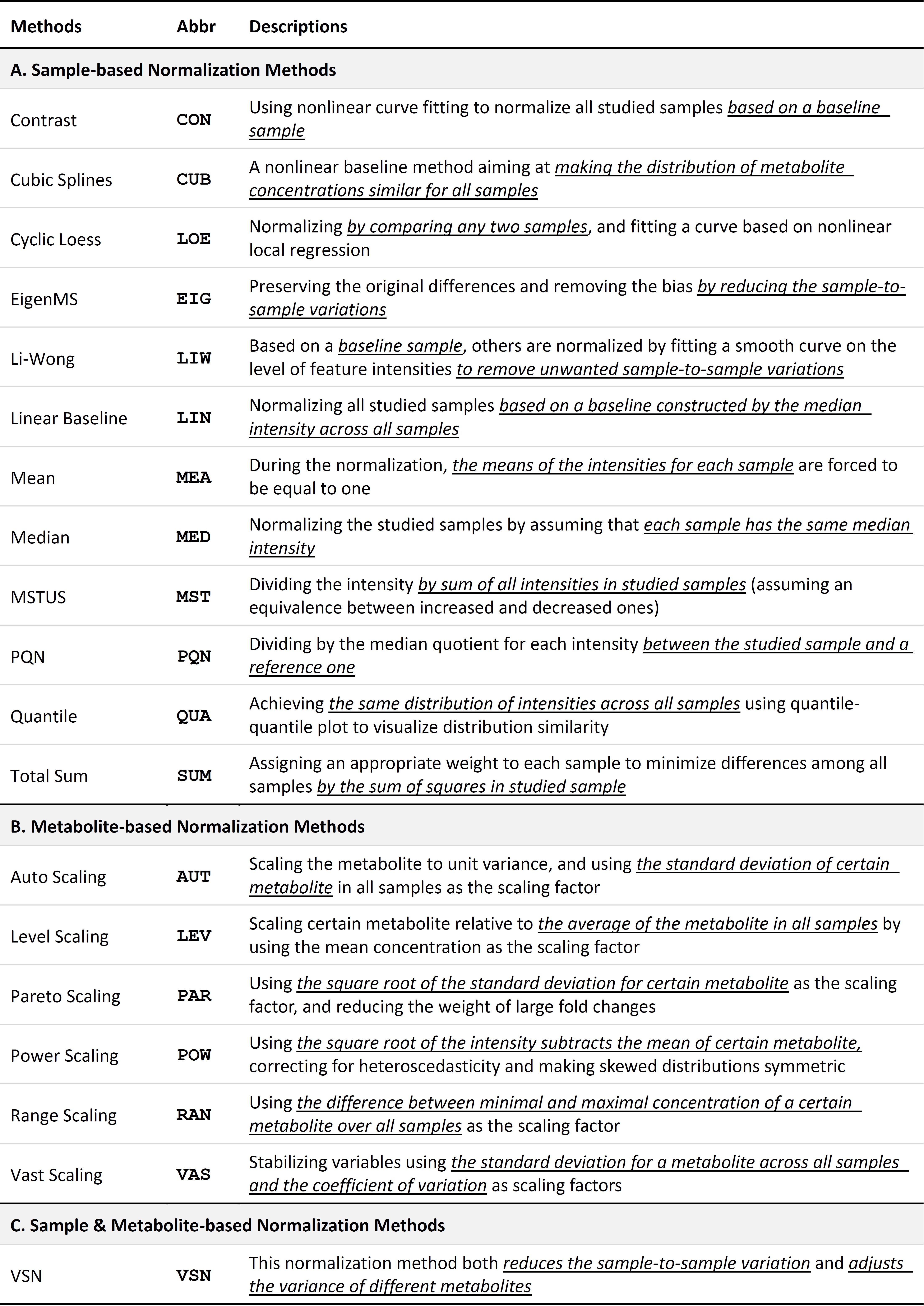
Normalization methods are widely applied for removing unwanted experimental/biological variation and technical error. These methods can be roughly divided into two categories: sample-based and metabolite-based (Xia J, et al. Nat Protoc. 6: 743-60, 2011). Herein, ≥19 methods are provided including (1) twelve sample-based normalization methods: Contrast, Cubic Splines, Cyclic Loess, EigenMS, Li-Wong, Linear Baseline, Mean Normalization, Median Normalization, MSTUS (MS Total Useful Signal), PQN (Probabilistic Quotient Normalization), Quantile and Total Sum; (2) six metabolite-based normalization methods: Auto Scaling, Level Scaling, Pareto Scaling, Power Scaling, Range Scaling and Vast Scaling; (3) one sample & metabolite based normalization methods: VSN (variance stabilizing normalization). For the majority of previous metabolomic studies, either a sample-based or a metabolite-based method is independently used for removing unwanted variations (Li XK, et al. Sci Transl Med. 10: eaat4162, 2018; Naz S, et al. Eur Respir J. 49: 1602322, 2017). But the combined normalization between a sample-based and metabolite-based methods is also found to be effective by a few recent metabolomic studies (Gao X, et al. Nature. 572: 397-401, 2019). Herein, this novel approach was recommended to discover the most appropriate normalization strategies that are consistently well-performing under all evaluation criteria. The detailed description of each method is shown in below.
Summary and Visualization of the Data after Data Normalization
- Visualization of Intensity after Normalization
- Visualization of Particular Metabolite after Normalization
Please input the serial number of metabolic feature
- Datasets after Normalization
Summary and Visualization of the Data after Data Normalization
- Visualization of Intensity after Normalization
- Visualization of Particular Metabolite after Normalization
Please input the serial number of metabolic feature
- Datasets after Normalization
Summary and Visualization of the Data after Data Normalization
- Visualization of Intensity after Normalization
- Visualization of Particular Metabolite after Normalization
Please input the serial number of metabolic feature
- Datasets after Normalization
Introduction to the Performance Evaluation Step of NOREVA
- Criterion A: Method’s Capability of Reducing Intragroup Variation among Samples
The performance of normalization methods could be assessed using method’s capability of reducing intragroup variation among samples (Chawade A, et al. J Proteome Res. 13: 3114-20, 2014). (1) Common measures of intragroup variability among samples include Pooled Median Absolute Deviation (PMAD) and Pooled Estimate of Variance (PEV) (Valikangas T, et al. Brief Bioinform. 19: 1-11, 2018). A lower value denotes more thorough removal of experimentally induced noise and indicates a better performance. (2) Principal Component Analysis (PCA) is used to visualize differences across groups (Chawade A, et al. J Proteome Res. 13: 3114-20, 2014). The more distinct group variations indicate better performance of the applied normalization method. (3) Relative Log Abundance (RLA) plot is used to measure possible variations, clustering tendencies, trends and outliers across groups or within group (De Livera AM, et al. Anal Chem. 84: 10768-76, 2012). Boxplots of RLA are used to visualize the tightness of samples across or within group(s). The median in plots would be close to zero and the variation around the median would be low.
- Criterion B: Method’s Effect on Differential Metabolic Analysis
Method’s effect on differential metabolic analysis is applied to assess the performance of normalization methods (Valikangas T, et al. Brief Bioinform. 19: 1-11, 2018). Differentiation among different groups based on differential metabolic markers is shown using k-means clustering algorithm (Jacob S, et al. Diabetes Care. 40: 911-9, 2017). Methods will be considered as well-performed when an obvious differentiation among different groups in clustering is achieved.
- Criterion C: Method’s Consistency of the Identified Markers among Different Datasets
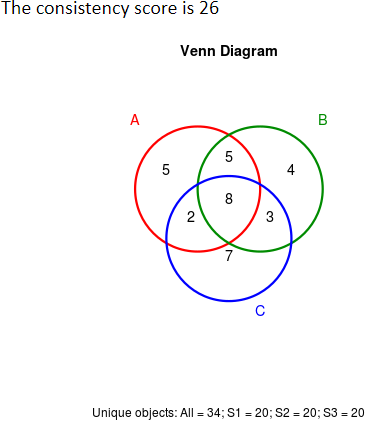
The performance of normalization methods could be assessed by method’s consistency of the identified metabolic markers among different datasets (Wang X, et al. Mol Biosyst. 11: 1235-40, 2015). Overlap of identified metabolic markers among different partitions is calculated using consistency score and the higher consistency score represents the more robust results in metabolic marker identification for that given dataset (Wang X, et al. Mol Biosyst. 11: 1235-40, 2015).
- Criterion D: Method’s Influence on Classification Accuracy
Method’s influence on classification accuracy is used to evaluate the performance of normalization methods (Risso D, et al. Nat Biotechnol. 32: 896-902, 2014). The classification accuracy is measured using ROC curve and AUC value based on support vector machine model (Gromski P S, et al. Metabolomics. 11: 684-95, 2015).
- Criterion E: Level of Correspondence between Normalized and Reference Data
The performance of normalization methods could be assessed using level of correspondence between normalized and reference data (Valikangas T, et al. Brief Bioinform. 32: 896-902, 2014). The performance of each method could be reflected by how well the log fold changes of normalized data corresponded to what were expected based on references including spike-in compounds and various molecules detected by quantitative analysis (Franceschi P, et al. J. Chemom. 26: 16-24, 2012). The preferred median in boxplot would be zero with minimized variations.
Summary and Visualization for Performance Evaluation from Multiple Perspectives
- Criterion A: Method’s Capability of Reducing Intragroup Variation among Samples
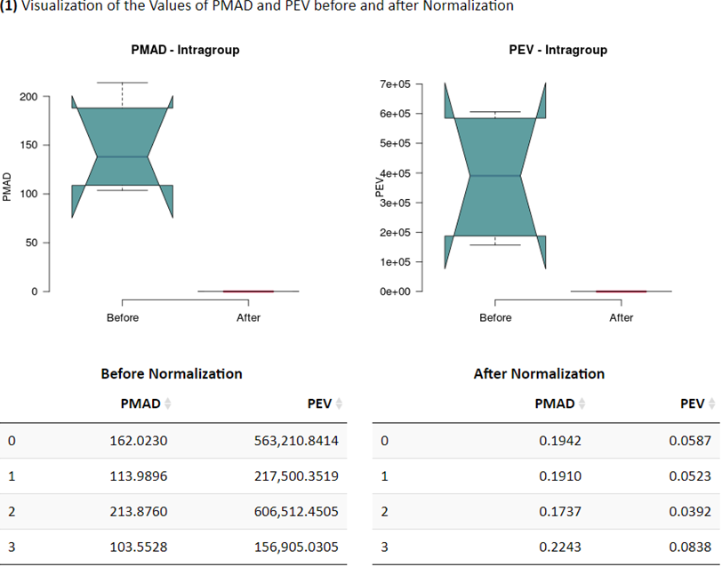
(1) Visualization of the Values of PMAD and PEV before and after Normalization
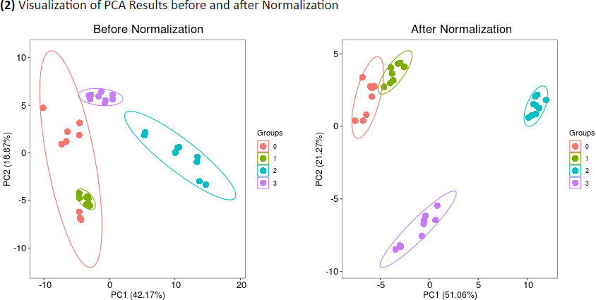
(2) Visualization of PCA Results before and after Normalization
(3) Visualization of the Results of Relative Log Abundance (RLA) after Normalization
- Criterion B: Method’s Effect on Differential Metabolic Analysis
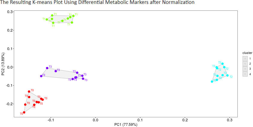
The Resulting K-means Plot Using Differential Metabolic Markers after Normalization
- Criterion C: Method’s Consistency of the Identified Markers among Different Datasets
- Criterion D: Method’s Influence on Classification Accuracy
- Criterion E: Level of Correspondence Between Normalized and Reference Data
(1) For this dataset, difference between metabolomics data and true marker estimates of log-fold-changes of means between two groups, that is, bias in metabolomics data when viewing true markers as the gold standard.
(2) Difference between metabolomics data and true marker estimates of log-fold-changes of standard deviation (SD) between two groups, that is, bias in metabolomics data when viewing true markers as the gold standard.
Summary and Visualization for Performance Evaluation from Multiple Perspectives
- Criterion A: Method’s Capability of Reducing Intragroup Variation among Samples
(1) Visualization of the Values of PMAD and PEV before and after Normalization
(2) Visualization of PCA Results before and after Normalization
(3) Visualization of the Results of Relative Log Abundance (RLA) after Normalization
- Criterion B: Method’s Effect on Differential Metabolic Analysis
The Resulting K-means Plot Using Differential Metabolic Markers after Normalization
- Criterion C: Method’s Consistency of the Identified Markers among Different Datasets
- Criterion D: Method’s Influence on Classification Accuracy
- Criterion E: Level of Correspondence Between Normalized and Reference Data
(1) For this dataset, difference between metabolomics data and true marker estimates of log-fold-changes of means between two groups, that is, bias in metabolomics data when viewing true markers as the gold standard.
(2) Difference between metabolomics data and true marker estimates of log-fold-changes of standard deviation (SD) between two groups, that is, bias in metabolomics data when viewing true markers as the gold standard.
- Criterion E: Level of Correspondence Between Normalized and Reference Data
(1) For this dataset, difference between metabolomics data and true marker estimates of log-fold-changes of means between two groups, that is, bias in metabolomics data when viewing true markers as the gold standard.
(2) Difference between metabolomics data and true marker estimates of log-fold-changes of standard deviation (SD) between two groups, that is, bias in metabolomics data when viewing true markers as the gold standard.
Table of Contents
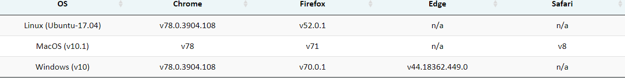
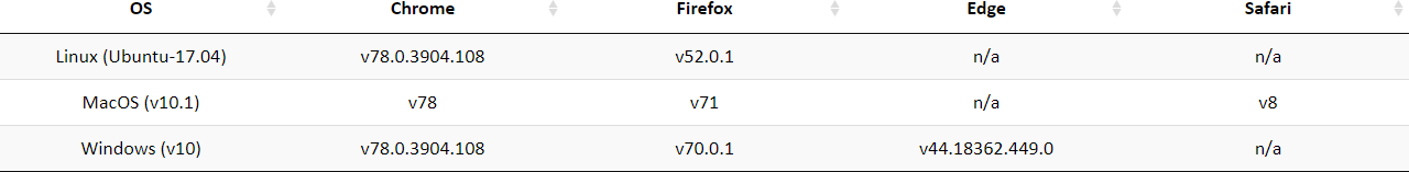
1. The Compatibility of Browser and Operating System (OS)
2. Required Formats of the Input Files
2.1 Time-course Metabolomic Data with Quality Control Samples (QCSs)
2.2 Time-course Metabolomic Data with Internal Standards (ISs)
2.3 Time-course Metabolomic Data without QCSs and ISs
2.4 Multi-class Metabolomic Data with QCSs
2.5 Multi-class Metabolomic Data with ISs
2.6 Multi-class Metabolomic Data without QCSs and ISs
2.7 Input File Containing the Reference Metabolites as Golden Standards
3. Step-by-step Instruction on the Usage of NOREVA
3.1 Uploading Your Customized Metabolomic Data or the Sample Data Provided in NOREVA
3.2 Data Preprocessing (Filtering & Imputation & Transformation)
3.3 Sample/Metabolite/IS-based Normalization Methods/Strategies
3.4 Evaluation of the Normalization Performance from Multiple Perspectives
4. A Variety of Methods for Data Preprocessing and Normalization
4.1 Filtering Methods
4.2 Missing-value Imputation Methods
4.3 Transformation Methods
4.4 Sample-based Normalization Methods
4.5 Metabolite-based Normalization Methods
4.6 Sample & Metabolite-based Normalization Method
4.7 IS-based Normalization Methods
NOREVA is powered by R shiny. It is free and open to all users with no login requirement and can be readily accessed by a variety of popular web browsers and operating systems as shown below.
In general, the file required at the beginning of NOREVA 2.0 analysis should be a sample-by-feature matrix in a csv format.
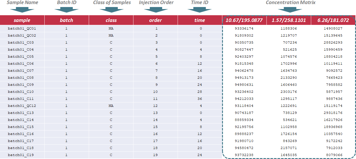
In this situation, the sample name, batch ID, class of samples, injection order and time ID are sequentially provided in the first 5 columns of input file. Names of these columns must be kept as "sample", "batch", "class", "order" and "time" without any changes during the entire analysis. The sample name is uniquely assigned according to the specified format ("batch & batch ID & _ & class name & injection order", e.g. "batch01_QC01"); the batch ID refers to different analytical blocks or batches, and is labeled with ordinal number, e.g., 1,2,3,…; the class of samples indicates 2 sample groups and QC samples (the name of sample groups is different, and QC samples are all labeled as "NA"); the injection order strictly follows the sequence of experiment; the time ID refers to time points of the experiment. Importantly, the first row must be a QC sample, and the last row also must be a QC sample. Sample data of this data type can be downloaded .
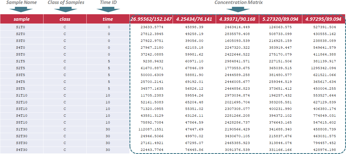
Under this circumstance, sample name, class of samples and time ID are required in the first 3 columns of the input file, and are kept as "sample", "class" and "time". The sample ID is uniquely assigned according to the specified format ("S & sample ID & T & Time ID", e.g., "S1T0"); The sample ID mentioned above is referred to different samples, and is labeled with ordinal number, e.g., 1,2,3. In the column of class of samples, "NA" is not labeled to any sample due to the absence of QC samples. The time ID refers to time points of experiment. In the following columns of the input file, metabolites’ raw intensities across all samples are further provided. Unique IDs of each metabolite are listed in the first row of the csv file. Sample data of this data type can be downloaded .
Under this circumstance, sample name, label name and time ID are required in the first 3 columns of the input file, and are kept as "sample", "label" and "time". The sample ID is uniquely assigned according to the specified format ("S & sample ID & T & Time ID", e.g., "S1T0"); The sample ID mentioned above is referred to different samples, and is labeled with ordinal number, e.g., 1,2,3. The label ID is referred to the property of samples, e.g., phenotype. The time ID referls to time points of the experiment. In the following columns of the input file, metabolites’ raw intensities across all samples are further provided. Unique IDs of each metabolite are listed in the first row of the csv file. Sample data of this data type can be downloaded .

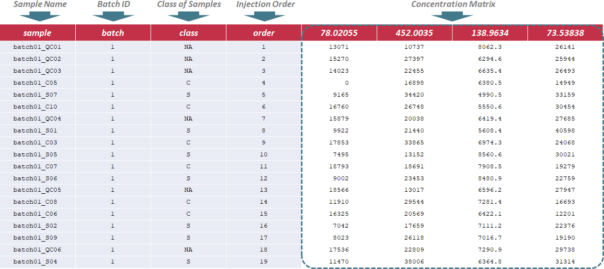
In this situation, the sample name, batch ID, class of samples and injection order are sequentially provided in the first 4 columns of input file. Names of these columns must be kept as "sample", "batch", "class" and "order" without any changes during the entire analysis. The sample name is uniquely assigned according to the specified format ("batch & batch ID & _ & Class & injection order", e.g., "batch01_QC01"); the batch ID refers to different analytical blocks or batches, and is labeled with ordinal number, e.g., 1,2,3,…; the class of samples indicates 2 sample groups and QC samples (the name of sample groups is different, and QC samples are all labeled as "NA"); the injection order strictly follows the sequence of the experiment. Importantly, the first row must be a QC sample, and the last row also must be a QC sample. Sample data of this data type can be downloaded .
Under this circumstance, only sample name and class of samples are required in the first 2 columns of the input file, and are kept as "sample name" and "label". In the column of class of samples, "NA" is not labeled to any sample due to the absence of QC samples. In the following columns of the input file, metabolites’ raw intensities across all samples are further provided. Unique IDs of each metabolite are listed in the first row of the csv file. Sample data of this data type can be downloaded .
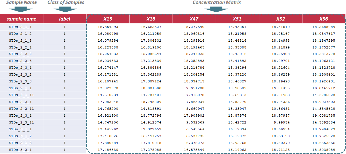
Under this circumstance, only sample name and label ID are required in the first 2 columns of the input file, and are kept as "sample name" and "label". In the column of label ID, "NA" is not labeled to any sample due to the absence of QC samples. The label ID is referred to the different classes of samples, and is labeled with ordinal number, e.g., 1,2,3. In the following columns of the input file, metabolites’ raw intensities across all samples are further provided. Unique IDs of each metabolite are listed in the first row of the csv file. Sample data of this data type can be downloaded .
To evaluate methods based on the last criterion, additional file providing information of the reference metabolites (e.g., spike-in compounds) is needed for further analysis. In this file, sample name and class of samples are required in the first 2 columns. Their names are provided as "sample name" and "label". The sample ID is also uniquely assigned according to users’ preference, and the class of samples indicates 2 sample groups of different names. The data format is the same for all data types, and the sample data for time-course studies can be downloaded .
This website is free and open to all users and there is no login requirement, and can be readily accessed by all popular web browsers including Google Chrome, Mozilla Firefox, Safari and Internet Explorer 10 (or later), and so on. Analysis and subsequent performance assessment are started by clicking on the "Analysis" panel on the homepage of NOREVA 2.0. The collection of web services and the whole process provided by NOREVA 2.0 can be summarized into 4 steps: (3.1) uploading metabolomics data, (3.2) data preprocessing, (3.3) data normalization and (3.4) performance evaluation. A report containing evaluation results is also generated and can be downloaded in the format of PDF, HTML and DOC. The flowchart below summarizes the flowchart of analyzing processes in NOREVA 2.0.

There are 3 radio checkboxes in STEP-1 on the left side of the Analysis page. Users can choose to upload their own metabolomics data or to directly load sample data. The type of the study and the type of the metabolomics data can also be selected in the remaining 2 radio checkboxes below. After selecting 3 corresponding radio checkboxes, datasets provided by the users for further analysis can be then directly uploaded by clicking "Browse". Preview of the uploaded data is subsequently provided on the web page. Moreover, users could process their data by uploading the raw data in a unified format.
6 sets of sample data are also provided in this step facilitating a direct access and evaluation of NOREVA 2.0. These sample data are all benchmark datasets collected from MetaboLights database developed by the European Bioinformatics Institute, which included (1) MTBLS403 dataset of time-course metabolomics study with QCSs: part of the dataset (3 time points are chosen from all time points, including 0, 12 and 36h) of a nontargeted metabolomics study on characterization of white tea metabolome. (2) MTSBL319 dataset of time-course metabolomics study with ISs: part of the dataset (gas toluene are selected from all stress conditions and mutant strains are selected from all gene knockouts, respectively) of a metabolomics study to elucidate any observable metabolic alterations during interactions of several strains of Pseudomonas putida (DOT-T1E, and its mutants DOT-T1E-PS28 and DOT-T1E-18) with the aromatic hydrocarbon toluene. And the time blocking (dosage of toluene) is the experiment factor in this dataset, which involves 0, 10 and 60 mins. (3) time-course metabolomics study without QCSs and ISs: part of the dataset of a study on the wound response of wild type Arabidopsis thaliana during a wounding time course (4 time points), based on LC-MS metabolite profile intensities from 8 different experimental conditions. This dataset is used as benchmark dataset for demonstrating that clustering and visualization capabilities can be used to identify relevant groups of markers (Meinicke P, et al. Algorithms Mol Biol. 3: 9, 2008). (4) MTBLS370 dataset of multi-class (N>1) metabolomics study with QCSs: part of the dataset (intracellular parts are selected from all organism parts) of a metabolomics study on Candida albicans and Staphylococcus aureus, which includes 18 samples from 3 classes of organisms and 11 QC samples. (5) MTBLS370 dataset of multi-class (N>1) metabolomics study with ISs: part of the dataset (culture supernatants are selected from all organism parts) of a metabolomics study on Candida albicans and Staphylococcus aureus, which includes 18 samples from 3 classes of organisms. (6) MTBLS159 dataset of multi-class (N>1) metabolomics study without QCSs and ISs: comprised of 4 classes of samples, which refer to the plasma samples obtained from DIO mice subjected to vehicle (water) treatment, or peptide treatment with humanin analog S14G (HNG), SHLP2 or MOTS-c (n = 6 per group). This set of data is the metabolomics profile of diet-induced obesity mice in response to human and small humanin-like peptide 2 treatment. By clicking the Load Data button, the sample dataset selected by the users can be uploaded for further analysis.
Data filtering, missing value imputation and data transformation are subsequently provided in this step. The filtering methods used here are the tolerance percentage of missing values and the tolerance of RSD. And 7 imputation methods frequently applied to treat missing value are covered, which include BPCA Imputation, Column Mean Imputation, Column median Imputation, Half of the Minimum Positive Value Imputation, KNN Imputation, SVD and Zero Imputation. Moreover, 2 transformation methods are adopted in NOREVA 2.0, which involve Cube Root Transformation, Log Transformation. A detailed explanation on each filtering, imputation and transformation method is provided in the Section 4 of this Manual. For data with QCSs, QCSs correct model should also be selected on the left side panel. After selecting or defining preferred methods or parameters, please proceed by clicking the "PROCESS" button, a summary of the processed data and plots of the intensity distribution before and after data manipulation are automatically generated. All resulting data and figures can be downloaded by clicking the corresponding "Download" button.
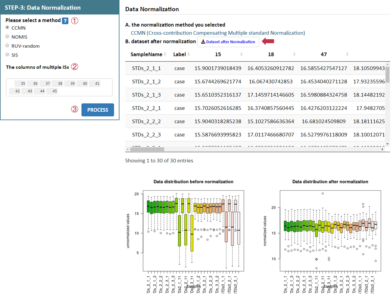
Data normalization is subsequently provided in this step. NOREVA 2.0 offers 12 sample-based, 6 metabolite-based ,1 sample and metabolite-based and 4 IS-based normalization methods for analyzing MS-based or NMR-based metabolomics data. A detailed explanation on each normalization method is provided in the Section 4 of this Manual.
For data with QCSs or without QCSs and ISs, users can select each combination of methods by selecting the 2 corresponding radio checkboxes indicating the sample-based or metabolite-based normalization methods in STEP-3 on the left side of the Analysis page. After selecting preferred methods, please proceed by clicking the PROCESS button, a summary of the processed data and plots of the intensity distribution before and after data normalization are automatically generated. All resulting data and figures can be downloaded by clicking the corresponding download button.
For data with ISs, IS-based normalization methods can be selected in the corresponding radio checkbox. The information of columns of multiple ISs is also provided by users.After selecting preferred method, please proceed by clicking the PROCESS button, a summary of the processed data and plots of the intensity distribution before and after data normalization are automatically generated. All resulting data and figures can be downloaded by clicking the corresponding download button.
5 well-established criteria for a comprehensive evaluation on the performance of normalization methods are provided in NOREVA 2.0, and each criterion is either quantitatively or qualitatively assessed by various metrics. These criteria include:
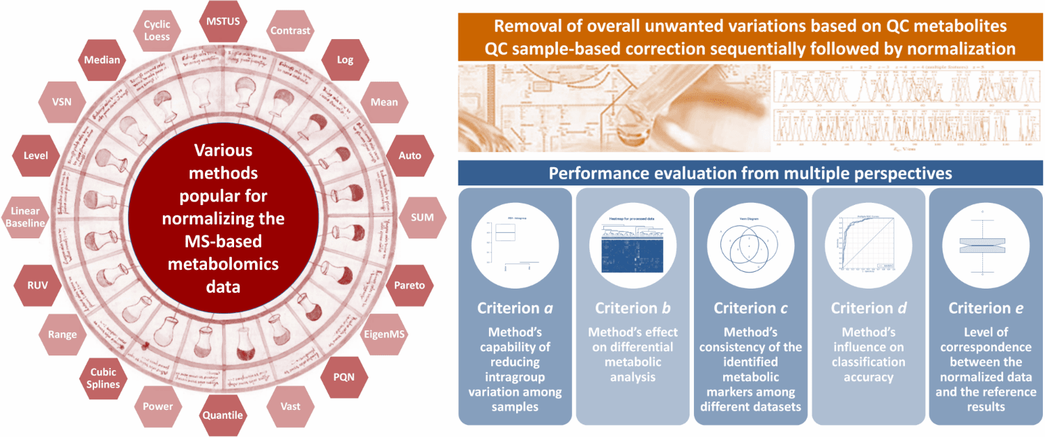
Common measures of intragroup variability including pooled median absolute deviation (PMAD) and pooled estimate of variance (PEV) are adopted under this criterion to evaluate variation between samples (Välikangas T, et al. Brief Bioinform. 19: 1-11, 2018). A lower value (illustrated by boxplots) of these two measures denotes more thorough removal of experimentally induced noise and indicates a better performance. Moreover, the principal component analysis (PCA) is also used to visualize differences across groups. The more distinct group variations indicate better performance of the applied normalization method. In addition, the relative log abundance (RLA) plots (De Livera AM, et al. Anal Chem. 84: 10768-76, 2012) used to measure possible variations, clustering tendencies, trends and outliers across groups or within group are also provided. Boxplots of RLA are used to visualize the tightness of samples across or within group(s). The median in boxplots would be close to zero and the variation around the median would be low (De Livera,A.M., et al. Metabolomics Tools for Natural Product Discovery: Methods and Protocols. 1055: 291-307, 2013).

K-means clustering is a commonly used method to partition data into several groups that minimizes variations in values within clusters (Jacob S, et al. Diabetes Care. 40: 911-9, 2017). First, samples are randomly assigned to one of a prespecified number of groups. Then, the mean value of the observations in each group is calculated, and samples are replaced into the group with the closest mean. Finally, the process mentioned above proceeds iteratively until the mean value of each group no longer changes (Jacob S, et al. Diabetes Care. 40: 911-9, 2017). Therefore, the plot of k-means clustering can be used to evaluate method’s effect on differential metabolic analysis. The more distinct group variations indicate better performance of the applied normalization method.
Under this criterion, a consistency score is defined to quantitatively measure the overlap of identified metabolic markers among different partitions of a given dataset (Wang X, et al. Mol Biosyst. 11: 1235-40, 2015). The higher consistency score represents the more robust results in metabolic marker identification for that given dataset.
(De Livera AM, et al. Anal Chem. 84: 10768-76, 2012; Risso D, et al. Nat Biotechnol. 32: 896-902, 2014; Piotr S. Gromski, et al. Metabolomics. 11: 684-95, 2015)
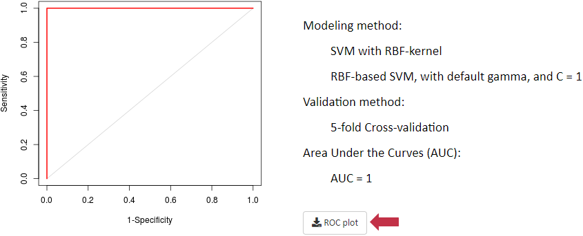
Under this situation, receiver operating characteristic (ROC) curve together with area under the curve (AUC) values based on support vector machine (SVM) are provided. First, differential metabolic features are identified by partial least squares discriminant analysis (PLS-DA). Second, the SVM models are constructed based on these differential features identified. After k-folds cross validation, a method with larger area under the ROC curve and higher AUC value is recognized as well performed (De Livera AM, et al. Anal Chem. 84: 10768-76, 2012; Risso D, et al. Nat Biotechnol. 32: 896-902, 2014; Piotr S. Gromski, et al. Metabolomics. 11: 684-95, 2015).
If this criterion is selected, an additional reference file providing information of golden standard metabolites should be uploaded as a csv file. The format of this file is described in the "Input File Containing Reference Metabolites as Golden Standards" section. Additional experimental data are frequently generated as references to validate or adjust prior result of metabolomics analysis (Pietro Franceschi, et al. J.Chemom. 26: 16-24, 2012). These references could be spike-in compounds and various molecules detected by quantitative analysis (Pietro Franceschi, et al. J.Chemom. 26: 16-24, 2012). Here, log fold changes (logFCs) of concentration between multiple groups are calculated, and the level of correspondence between normalized data and references is then estimated. The performance of each method could be reflected by how well the logFCs of normalized data corresponded to what are expected based on references (Välikangas T, et al. Brief Bioinform. 19: 1-11, 2018).

- Tolerable Percent of Missing Values.Metabolomics data is filtered when the tolerable percent of missing values in each metabolite is over the set cutoff. The cutoff of the tolerable percent of missing values could be set by users and default value is 0.2 based on "80% rule" in metabolomics (Chen J, et al. Anal Chem. 89: 5342-8, 2017).
- Tolerance of Relative Standard Deviation (RSD). RSD is the absolute measurement of batch-to-batch variation and a lower RSD indicates better reproducibility of the feature (Dunn WB, et al. Nat Protoc. 6: 1060-83, 2011). The metabolite is deleted when its RSD across QCs is higher than a threshold which is defined by the user (default 30%).
4.2 Missing-value Imputation Methods
- BPCA Imputation (Bayesian Principal Component Analysis Imputation). BPCA imputation imputes missing data with the values obtained from Bayesian principal component analysis regression (Oba S, et al. Bioinformatics. 19: 2088-96, 2003). The number of principal components to calculate could be set by users and is 3 by default.
- Column Mean Imputation. Column mean imputation method imputes missing values with the mean value of non-missing values in the corresponding metabolite (Huan T, et al. Anal Chem. 87: 1306-13, 2015).
- Column Median Imputation. Column median imputation method imputes missing values with the median value of non-missing values in the corresponding metabolite (Huan T, et al. Anal Chem. 87: 1306-13, 2015).
- Half of the Minimum Positive Value. The missing value could be imputed using the half of the minimum positive value in all metabolomics data (Taylor SL, et al. Brief Bioinform. 18: 312-20, 2017).
- KNN Imputation. KNN imputation (K-nearest Neighbor Imputation) method aims to find k metabolites of interest which are similar to the metabolites with missing value. The similarity is measured by Euclidean distance and the missing value is imputed by the weighted average of those k metabolites (Tang J, et al. Brief Bioinform. doi: 10.1093/bib/bby127). 4 parameters could be set by users: (1) The default number of Neighbors is set 10;(2) missing value is imputed using the overall mean per sample if the maximum percent missing data allowed in any row is more than the cutoff (default 0.5); (3) the program halts and reports an error if the maximum percent missing data allowed in any column is more than the cutoff (default 0.8); (4) the largest block of features imputed using the knn algorithm was set 1500 by default.
- SVD Imputation. The fundamental principle of SVD (Singular Value Decomposition) imputation method is to analyze the principle components that represent the entire matrix information and then to estimate the missing values by regressing against the principle components (default 3) (Gan X, et al. Nucleic Acids Res. 34: 1608-19, 2006).
- Zero Imputation. Zero Imputation method simply replaces all missing values with zero (Gromski PS, et al. Metabolites. 4: 433-52, 2014).
- Cube Root Transformation. Cube root transformation is employed to improve the normality distribution of simple count data (Ho EN, et al. Drug Test Anal. 7: 414-9, 2015).
- Log Transformation. Log Transformation is a nonlinear conversion of data to decrease heteroscedasticity and obtain a more symmetric distribution prior to statistical analysis (Purohit PV, et al. OMICS. 8: 118-30, 2004).
- QC Sample Correction and Parameter Setting of Regression Model. The correction strategy based on multiple QC samples is a popular method to evaluate the signal drift and other systematic noise through mathematical algorithms in metabolomics studies (Luan H, et al. Anal Chim Acta. 1036: 66-72, 2018). The regression model for QC-RLSC including Nadaraya-Watson estimator, local linear regression and local polynomial fits could be defined by users.
- Contrast. Contrast is a sample-based normalization method where a baseline sample is selected to which other samples are normalized by fitting a nonlinear smooth curve (Astrand M, et al. Comput Biol. 10: 95-102, 2003; Kohl SM, et al. Metabolomics. 8: 146-60, 2012). The method achieves its efficacy by three steps, including change of basis, fitting the normalizing curve and normalizing the samples (Astrand M, et al. Comput Biol. 10: 95-102, 2003). The intensities are logged and further transformed into the contrast space using an orthonormal matrix. This method has been used to process the LC/MS based metabolomics data and to correct for unwanted experimental or biological variations and technical errors (Li B, et al. Sci Rep. 6: 38881, 2016).
- Cubic Splines. Cubic Splines is categorized as a sample-based normalization method using the nonlinear baseline which aims to make the distribution of metabolite concentrations (geometric or arithmetic mean) among all samples comparable (Saccenti E, et al. J Proteome Res. 16: 619-34, 2017Kohl SM, et al. Metabolomics. 8: 146-60, 2012). After change of basis, a number of evenly distributed quantiles across all samples are collected to fit a smooth cubic spline. Furthermore, the spline function generator is applied to fit the parameters of the cubic spline, which uses a set of interpolated splines. This method has been utilized in an automated DIMS metabolomics workflow to characterize and correct for batch variation(Kirwan JA, et al. Anal Bioanal Chem. 405: 5147-57, 2013).
- Cyclic Loess. Cyclic Loess is also referred as cyclic locally weighted regression, aiming to fit a normalization curve based on nonlinear local regression and to normalize all studied samples via comparing any two samples based on MA-plots which constitute logged Bland-Altman plots (Kohl SM, et al. Metabolomics. 8: 146-60, 2012). To be more specific, the process of LOE is described below. The logged peak intensity ratio is compared to their corresponding average feature by feature, and a normalization curve based on nonlinear local regression which is subtracted from the original values is fitted. If there are more than two spectra to be normalized, the method mentioned above is carried out similarly by iterating in pairs for all possible combinations (Kohl SM, et al. Metabolomics. 8: 146-60, 2012). This method has been used to large-scale LC-MS-based metabolomics profiling and is discovered to be able to remove the systematic effect (Ejigu BA, et al. OMICS. 17: 473-85, 2013).
- EigenMS. EigenMS is defined as a sample-based normalization method which removes the deviations via reducing the sample-to-sample variations of unknown complexity while preserves the original differences simultaneously (Ejigu BA, et al. OMICS. 17: 473-85, 2013; Karpievitch YV, et al. PLoS One. 9: e116221, 2014; Karpievitch YV, et al. Bioinformatics. 25: 2573-80, 2009). This method is an adaption of surrogate variable analysis of Leek and Storey (Leek JT, et al. PLoS Gene. 3: 1724-35, 2007), which uses singular value decomposition to reduce biases in metabolomics peak intensities. EIG can be broken down into three steps, including preserving the original differences with an ANOVA model, determining bias trends based on singular value decomposition, and elimination of the bias trends which is estimated by a permutation test. This method has been adopted in processing LC-MS-based metabolomics data to detect and correct for any systematic bias (Karpievitch YV, et al. PLoS One. 9: e116221, 2014) and has also been revealed that it outperforms to other existing alternatives by both large-scale calibration measurements and simulations (Karpievitch YV, et al. Bioinformatics. 25: 2573-80, 2009).
- Linear Baseline. Linear Baseline reduces the sample-to-sample variations by using a scaling factor to map each spectrum to a linear baseline derived from calculating the median intensity of all samples (Kohl SM, et al. Metabolomics. 8: 146-60, 2012). The scaling factor of each spectrum is determined by computing the ratio of the mean intensity of the baseline to the mean intensity of each spectrum. And the intensity of each spectrum is multiplied by its corresponding scaling factor. The drawback of LIN is that the assumption of a linear correlation among spectra may be oversimplified. It has been utilized in preprocessing LC–MS metabolomics data to correct for systematic variation and to scale the data so that different samples in a study can be compared with each other (Sandra Castillo, et al. Chemometr intel lab. 1: 23-32, 2011).
- Li-Wong. Li-Wong is a sample-based normalization method where a baseline spectrum is selected and other spectra are normalized by fitting a smooth curve on the level of feature intensities that only uses a subset of features (Astrand M, et al. J Comput Biol. 10: 95-102, 2003). The subset of features with small absolute rank differences is selected prior to fitting the curve based on the assumption that features corresponding to unregulated metabolites have similar intensity ranks in two spectra can be expected to determine a reliable normalization curve (Astrand M, et al. J Comput Biol. 10: 95-102, 2003). To be more specific, the normalization process is carried out by scatter plots with the baseline spectrum (x-axis) and other spectra to be normalized (y-axis). Then, the dataset should align along the diagonal y=x (Kohl SM, et al. Metabolomics. 8: 146-60, 2012). This method has been used to remove unwanted sample-to-sample variation in NMR-based normalization analysis (Kohl SM, et al. Metabolomics. 8: 146-60, 2012).
- Mean Normalization. Mean Normalization is a sample-based normalization method to eliminate background effect in which the means of the intensities for each sample are forced to be equal to one another (Ejigu BA, et al. OMICS. 17: 473-85, 2013; Andjelkovic V, et al. Plant Cell Rep. 25: 71-9, 2006). This method is used to force the means of the intensities for each sample to be the same value, and therefore to make the samples comparable to each other. This method has been applied to process large-scale LC-MS-based metabolomics dataset and is discovered to be able to eliminate background effect (Ejigu BA, et al. OMICS. 17: 473-85, 2013).
- Median Normalization. Median Normalization is one of the commonly used sample-based normalization methods which do not take any internal standards, normalizing each sample to make the median of the metabolite abundances across samples equal to each other (Wang W, et al. Anal Chem. 75: 4818-26, 2003). This method is considered to be more practical than the normalization to a total sum (Crawford, L. R., et al. Anal Chem. 40: 1464-69, 1968), especially under the condition where several saturated abundances may be related to some of the factors of interest. This method has been adopted in a popular web server for metabolomics data analysis and interpretation (Xia J, et al. Nucleic Acids Res. 37: W652-60, 2009).
- MS Total Useful Signal (MSTUS). MS Total Useful Signal (MSTUS), also referred as MS total useful signal, is a sample-based normalization method where the intensity of each spectrum is divided by the sum of intensities of all spectra based on the assumption that there is an equivalence between increased intensities and decreased intensities (Saccenti E, et al. J Proteome Res. 16: 619-34, 2017; Warrack BM, et al. J Chromatogr B Analyt Technol Biomed Life Sci. 877: 547-52, 2009). The drawback of MSTUS is that the assumption may be questionable because an increase of the intensity of one metabolite is not necessarily associated with a decrease of the intensity of another metabolite (Saccenti E, et al. J Proteome Res. 16: 619-34, 2017). MSTUS has been recommended to be used as a normalization strategy for urinary metabolomics analysis, which equivalently improves the differentiation between the dose groups and therefore facilitates detection of statistically significant changes in the urine samples (Warrack BM, et al. J Chromatogr B Analyt Technol Biomed Life Sci. 877: 547-52, 2009).
- Probabilistic Quotient (PQN). Probabilistic Quotient (PQN) is a sample-based normalization method which assumes that biologically interesting concentration changes influence only parts of the spectrum, while dilution effects affect all metabolite signals (Emwas AH, et al. Metabolomics. 14: 31, 2018). PQN achieves its efficacy by 3 main steps (Emwas AH, et al. Metabolomics. 14: 31, 2018) : (1) the calculation of a reference spectrum (median or baseline) prior to the integral normalization of each spectrum; (2) the calculation of the variable quotient of a given test spectrum and the reference spectrum; (3)the division of all variables of the test spectrum by the estimation of the mean quotients. This method has been reported to act as a robust strategy to account for dilution of complex biological mixtures when applied in 1H NMR metabolomics analysis (Dieterle F, et al. Anal Chem. 78: 4281-90, 2006).
- Quantile. Quantile is a sample-based normalization method which aims to make the distribution of metabolite concentrations across all of the samples to be the same (Bolstad BM, et al. Bioinformatics. 19: 185-93, 2003). The distribution similarity of metabolite concentrations is visualized in this method by employing the quantile-quantile plot (Kohl SM, et al. Metabolomics. 8: 146-60, 2012). And QUA is supported by the hypothesis that any two metabolomics data vectors are the same if the quantile-quantile plot is a straight diagonal line (Bolstad BM, et al. Bioinformatics. 19: 185-93, 2003). This method has been recommended as a robust normalization strategy to process 1D 1H metabolomics data of urinary biofluids (Emwas AH, et al. Metabolomics. 14: 31, 2018).
- Total Sum Normalization. Total Sum Normalization is another most commonly used sample-based normalization method to reduce sample-to-sample variations which normalizes the metabolite concentrations by assigning an appropriate weight to the sample. After the normalization relying on the self-averaging property, the sum of squares of all abundances in a sample equals to each other in the studied data (De Livera AM, et al. Anal Chem. 87: 3606-15, 2015). So far, this method has been widely used to serve as a normalization strategy to correct for urinary output in HPLC-HRTOFMS metabolomics (Vogl FC, et al. Anal Bioanal Chem. 408: 8483-93, 2016).
- Auto Scaling. Auto Scaling is also referred as unit variance scaling, which is a metabolite-based normalization method to adjust metabolite variances. AUT achieves its efficacy by using the standard deviation as scaling factor to scale all of the metabolic signals (Kohl SM, et al. Metabolomics. 8: 146-60, 2012; Hu, C., et al. Anal Chem. doi: 10.1016/j.trac.2013.09.005). Metabolites are comparably scaled to unit variance based on the assumption that all metabolites are equally important. After auto scaling, the standard deviation equals value one (Kohl SM, et al. Metabolomics. 8: 146-60, 2012). Auto scaling has been used in MS-based metabolomics analysis to contribute to the diagnosis of the bladder cancer and urinary nucleoside biomarker identification from urogenital cancer patients (Struck W, et al. J Chromatogr A. 1283: 122-31, 2013).
- Level Scaling. Level Scaling is categorized as a metabolite-based normalization method in which metabolic signal variations are transformed to variations relative to the mean metabolic signal. In this case, the data are changed to values in percentages relative to the mean concentration after level scaling (van den Berg RA, et al. BMC Genomics. 7: 142, 2006) This method is especially applicable to preprocess the data in which huge relative variations are of great interest and to discover biomarkers concern about relative response (van den Berg RA, et al. BMC Genomics. 7: 142, 2006). A typical disadvantage of this method is amplified measurement errors. Be similar to auto scaling, level scaling has also been applied to discover urinary nucleoside biomarkers of urogenital cancer patients in MS-based metabolomics analysis (Struck W, et al. J Chromatogr A. 1283: 122-31, 2013).
- Pareto Scaling. Pareto Scaling uses the square root of the standard deviation of the corresponding metabolite as the scaling factor to reduce the weight of the large fold changes in metabolite signals, and is categorized as a metabolite-based normalization method (Eriksson L, et al. Anal Bioanal Chem. 380: 419-29, 2004). The capability of reducing large fold changes of pareto scaling is more powerful than auto scaling, while the dominant weight of extremely large fold changes may still be retained (Kohl SM, et al. Metabolomics. 8: 146-60, 2012). Therefore, the main drawback of pareto scaling is its sensitivity to the extremely large fold changes (van den Berg RA, et al. BMC Genomics. 7: 142, 2006). Pareto scaling has been adopted to serve as a data preprocessing strategy to eliminate the mask effect for metabolomics data analysis (Yang J, et al. Front Mol Biosci. 2: 4, 2015).
- Power Scaling. Power Scaling is a metabolite-based normalization method which targets to correct for heteroscedasticity and pseudo scaling (van den Berg RA, et al. BMC Genomics. 7: 142, 2006). Compared to the log transformation, power scaling adopts the similar transformation process, but power scaling has no problems to deal with zero values while not able to make multiplicative effects additive (van den Berg RA, et al. BMC Genomics. 7: 142, 2006). The obvious advantage of this method is that the choice for the corresponding square root is arbitrary (van den Berg RA, et al. BMC Genomics. 7: 142, 2006). This method has been used in mass spectrometry-based serum metabolic profiling and studying their alterations in colorectal cancer (Leichtle AB, et al. Metabolomics. 8: 643-53, 2012).
- Range Scaling. Range Scaling is a metabolite-based normalization method which takes the biological range (the variation between the maximum and the minimum intensity of a certain metabolite) as the scaling factor and divides the measured intensity by the scaling factor defined above (van den Berg RA, et al. BMC Genomics.7: 142, 2006; Smilde AK, et al. Anal Chem. 77: 6729-36, 2005). Obviously, all intensities are put on an equal footing and the variation level for metabolites are treated equally (Smilde AK, et al. Anal Chem. 77: 6729-36, 2005). The advantage of the method is that the relative concentration for each metabolite is rendered by removing instrumental response factor (Smilde AK, et al. Anal Chem. 77: 6729-36, 2005). However, the drawback of range scaling is its sensitivity to outliers because it only adopts two values to estimate the biological range (van den Berg RA, et al. BMC Genomics.7: 142, 2006). Range scaling has been used to fuse MS-based metabolomics data and leads to a comprehensive view on the metabolome of an organism or biological system (Smilde AK, et al. Anal Chem. 77: 6729-36, 2005).
- Vast Scaling. Vast Scaling is defined as a metabolite-based normalization method which weights each metabolite based on a metric of its stability and is an extension of auto scaling (Keun, H. C., et al. Anal Chem Acta.490: 265-76, 2003). This method chiefly focuses on the stable metabolites which do not show significant variation and is not suitable to normalize large induced variation without group structure (van den Berg RA, et al. BMC Genomics.7: 142, 2006). Vast scaling is considered to be stable and robust (Gromski, P. S., et al. Metabolomics.11: 684-95, 2014) has been adopted in unsupervised and supervised metabolomics analysis to enhance multivariate models used for classification and biomarker identification (Keun, H. C., et al. Anal Chem Acta.490: 265-76, 2003; Gromski, P. S., et al. Metabolomics.11: 684-95, 2014).
- VSN. VSN is a special normalization method based on both samples and metabolites. As a consequence, it is able to adjust the variations of different samples and remove the metabolite-to-metabolite variation (Hochrein J, et al. J Proteome Res.14: 3217-28, 2015). It is also a non-linear method which aims to make the variance constant over the entire data range (Kohl SM, et al. Metabolomics.8: 146-60, 2012; Huber W, et al. Bioinformatics.18: S96-104, 2002). When dealing with small intensities, it keeps variance unchanged by performing the linear transformation behavior. For large intensities, it uses the inverse hyperbolic sine to remove heteroscedasticity (Kohl SM, et al. Metabolomics.8: 146-60, 2012). This method is originally designed to normalize single and two-channel microarray data (Kultima K, et al. Mol Cell Proteomics.8: 2285-95, 2009), and currently gradually used in GC/MS-based metabolic profiling of liver tissue during early cancer development (Ibarra R, et al. HPB Surg.2014: 310372, 2014). VSN is also adopted to preprocess ultra-performance LC-MS urinary metabolic profiling for improved information recovery (Veselkov, K. A., et al. HPB Surg.83: 5864-72, 2011).
- Cross-Contribution Compensating Multiple Standard Normalization. Cross-Contribution Compensating Multiple Standard Normalization (CCMN) is applicable to monitor systematic error from randomized and designed experiments using multiple internal standards (Redestig H, et al. Anal Chem.81: 7974-80, 2009). CCMN compensates for systematic cross-contribution effects that can be traced back to a linear association with experimental design (Redestig H, et al. Anal Chem.81: 7974-80, 2009), and is superior at purifying the signal of interest using multiple internal standards (Redestig H, et al. Anal Chem.81: 7974-80, 2009). But care needs to be taken when normalizing the data using the factors of interest prior to carrying out unsupervised analysis (De Livera AM, et al. Anal Chem.87: 3606-15, 2015). CCMN is mainly aimed at MS-based metabolomics data and its inclusion will improve the precision of current metabolite profiling protocols (Jauhiainen A, et al. Bioinformatics.30: 2155-61, 2014).
- Normalization using Optimal Selection of Multiple Internal Standards. Normalization using Optimal Selection of Multiple Internal Standards (NOMIS) finds optimal normalization factor to remove unwanted systematic variation using variability information from multiple internal standard compounds (Sysi-Aho M, et al. BMC Bioinformatics.8: 93, 2007). NOMIS method can select best combinations of standard compounds for normalization using multiple linear regression and remove all correlations with the standards (Redestig H, et al. Anal Chem.81: 7974-80, 2009). This method has a superior ability to reduce variability across the full spectrum of metabolites (Sysi-Aho M, et al. BMC Bioinformatics.8: 93, 2007). Moreover, the NOMIS method can be used in both supervised and unsupervised analysis (De Livera AM, et al. Anal Chem.87: 3606-15, 2015). Now NOMIS method has been used to normalize LC/MS-based metabolomics data (Sysi-Aho M, et al. BMC Bioinformatics.8: 93, 2007).
- Remove Unwanted Variation-Random. Remove Unwanted Variation-Random (RUV-random) is based on a linear mixed effects model utilizing quality control metabolites to obtain normalized data in metabolomics experiments (De Livera AM, et al. Anal Chem.87: 3606-15, 2015). RUV-random method attempts to remove overall unwanted variation. RUV-random accommodates unwanted biological variation and retains the essential biological variation of interest. Moreover, the unwanted variation component from any undetected experimental or biological variability can be removed (De Livera AM, et al. Anal Chem.87: 3606-15, 2015). This method is applicable in both supervised and unsupervised analysis (De Livera AM, et al. Anal Chem.87: 3606-15, 2015). RUV-random is used for removing unwanted variation for MS-based metabolomics data.
- Single Internal Standard. Single Internal Standard (SIS) provides a normalized data matrix by subtracting the log metabolite abundance of a single internal standard from the log abundances of the metabolites in each sample (De Livera AM, et al. Anal Chem.84: 10768-76, 2012; Jonas Gullberg, et al. Anal biochem. doi: 10.1016/j.ab.2004.04.037, 2004). The SIS method assumes that every metabolite in a sample is subject to the same amount of unwanted variation and they can be simply measured by a single internal standard (De Livera AM, et al. Anal Chem.84: 10768-76, 2012). However, the use of a single internal standard may result in highly variable normalized values, which depend on the internal standard (De Livera AM, et al. Anal Chem.84: 10768-76, 2012). SIS method has been used to identify factors influencing extraction and derivatization of Asrabidopsis thaliana samples in the GC/MS-based metabolomics analysis (Jonas Gullberg, et al. Anal biochem. doi: 10.1016/j.ab.2004.04.037, 2004).
![]() @ ZJU
@ ZJU
Please feel free to visit our website at https://idrblab.org

Dr. Qingxia Yang (yangqx@cqu.edu.cn)
Dr. Yunxia WANG (lfwyx@zju.edu.cn)
Dr. Ying ZHANG (21919020@zju.edu.cn)
Dr. Fengcheng LI (lifengcheng@zju.edu.cn)
Prof. Feng ZHU* (zhufeng@zju.edu.cn)


Address
College of Pharmaceutical Sciences,
Zhejiang University,
Hangzhou, China
Postal Code: 310058

Phone/Fax