It is free and open to all users with no login requirement and can be readily accessed by a variety of popular web browsers and operating systems as shown below.

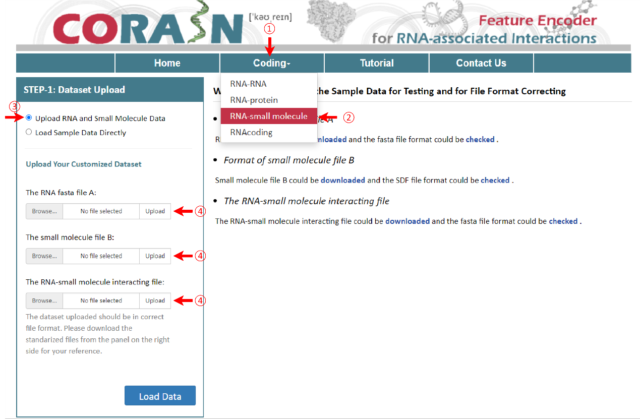
In general, the files required at the beginning of CORAIN analysis should be the FASTA files of RNA or protein and the sdf files of little molecules.

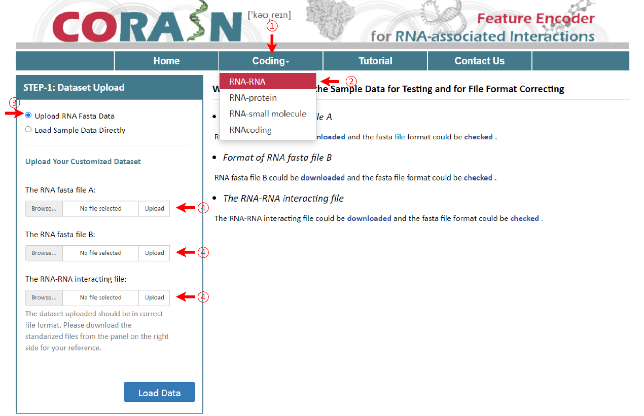
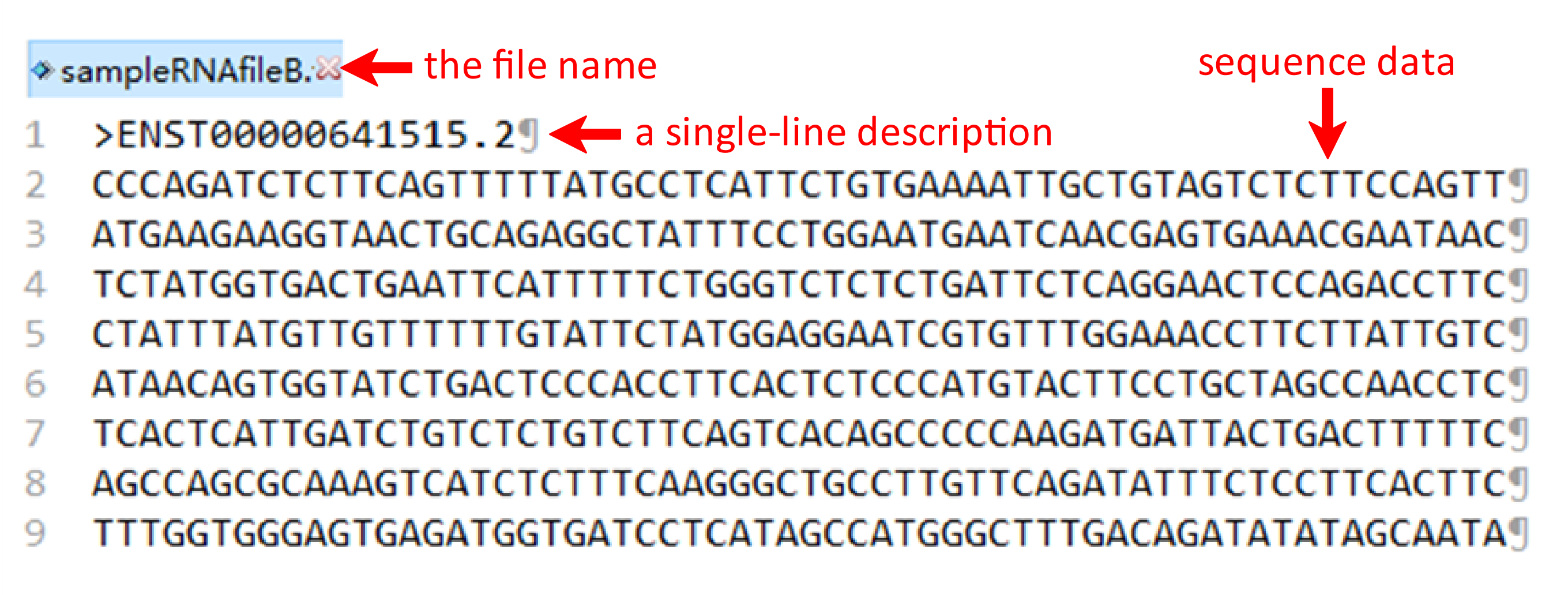
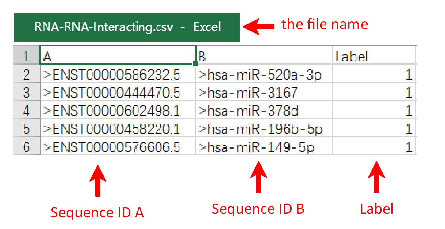
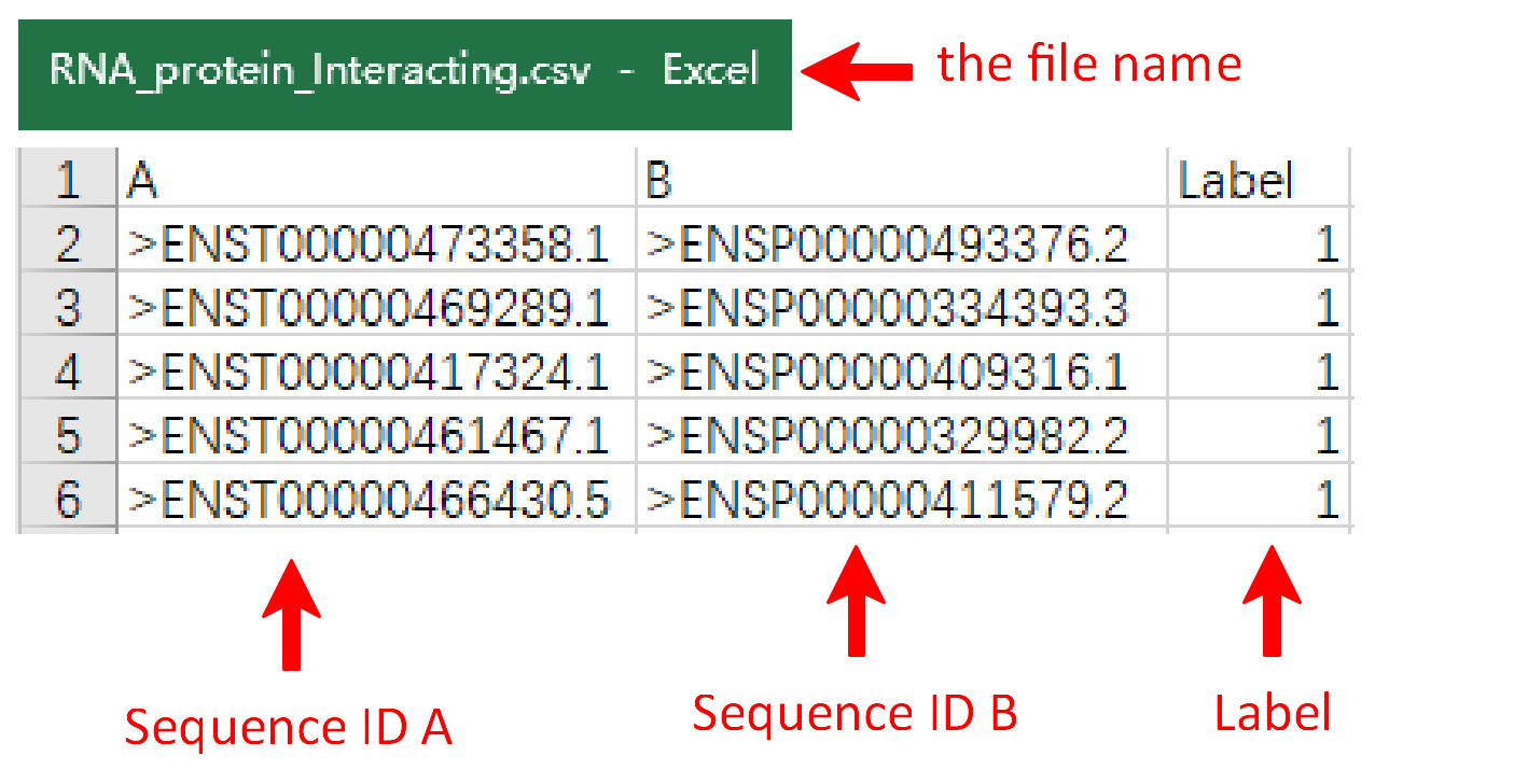
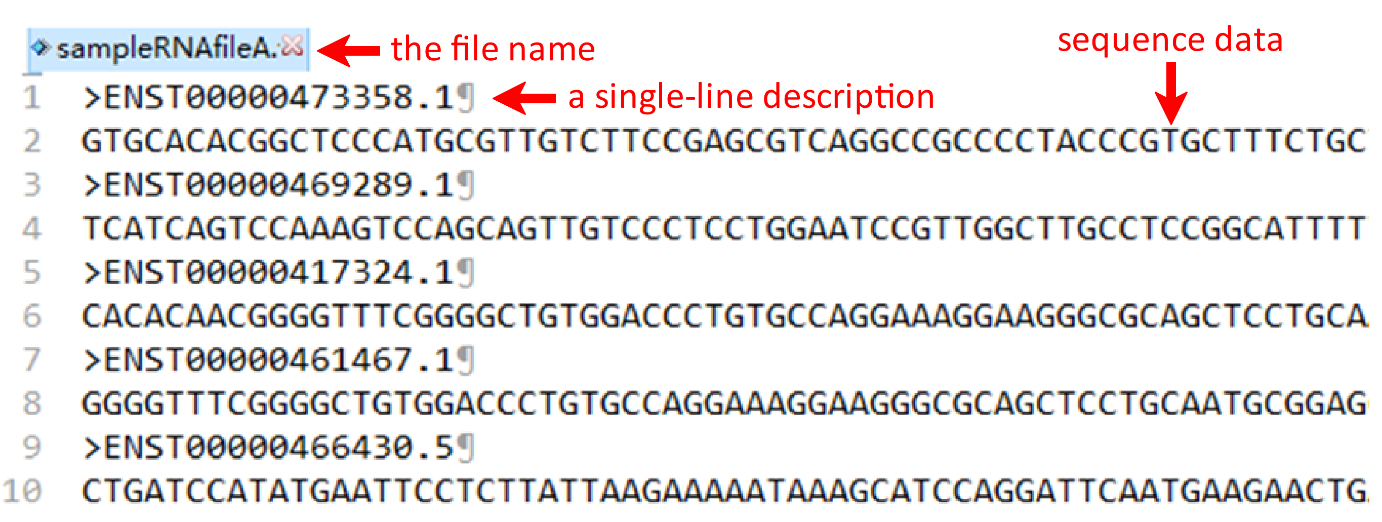
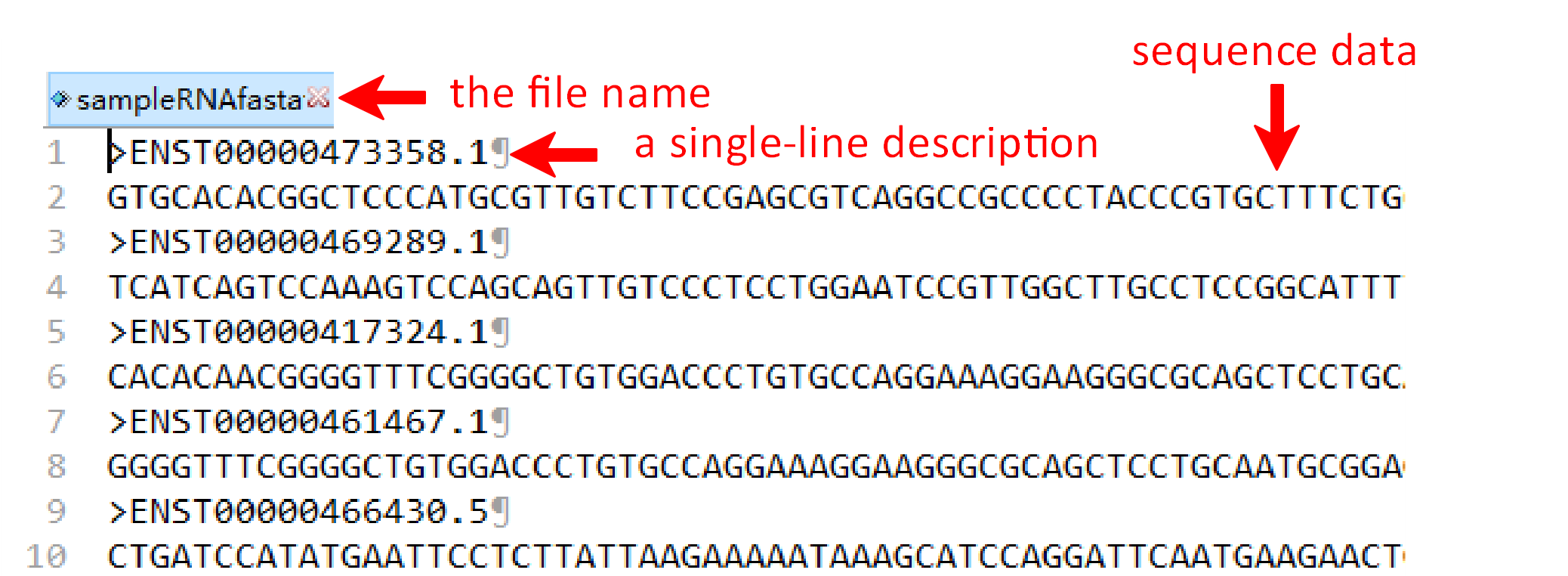
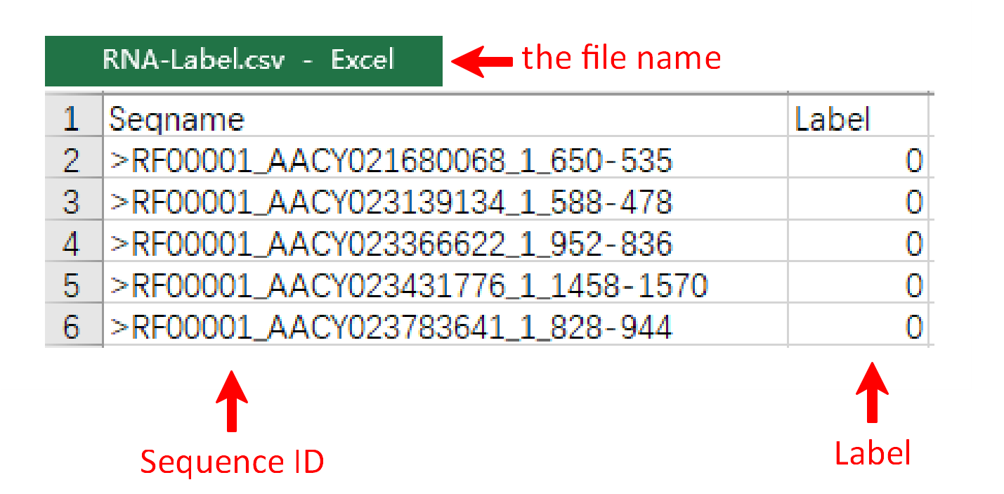
Under this circumstance, three files including RNA fasta file A, RNA fasta file B and the RNA-RNA interacting file should be uploaded. It's important to note that the names of RNA fasta files must end with ‘A’ or ‘B’, such as ‘sampleRNAfileA.fasta’ and ‘sampleRNAfileB.fasta’. A sequence in FASTA format begins with a single-line description, followed by lines of sequence data. The definition line (defline) is distinguished from the sequence data by a greater-than (>) symbol at the beginning. The word following the ">" symbol is the identifier of the sequence, and the rest of the line is the description (optional). For the RNA-RNA interacting file, it must be csv format and its name can only be ‘RNA-RNA-Interacting.csv’. In the RNA-RNA interacting file, the sequence ID of RNA files A and B are required in the first and second columns, while the third column is the label which the column name can’t be changed. There are sample RNA fasta file A and B and a sample RNA-RNA interacting file below.

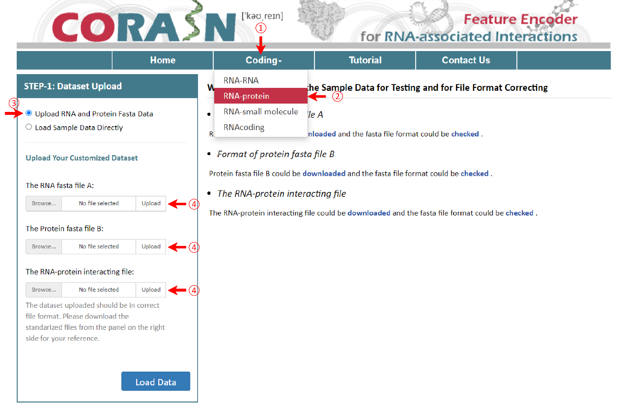
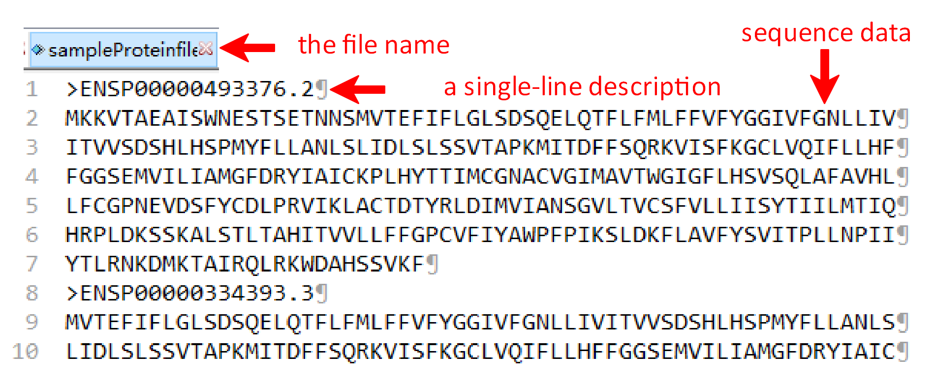
Similar to the above, three files including RNA fasta file A, protein fasta file B and the RNA-protein interacting file should be uploaded. It is noteworthy that the file A should be the RNA fasta file and the file B should be the protein fasta file, same ended with ‘A’ or ‘B’, such as ‘sampleRNAfileA.fasta’ and ‘sampleProteinfileB.fasta’. The RNA-protein interacting file can only be named as ‘RNA-Protein-Interacting.csv’ and the last column’s name must be the ‘Lable’.

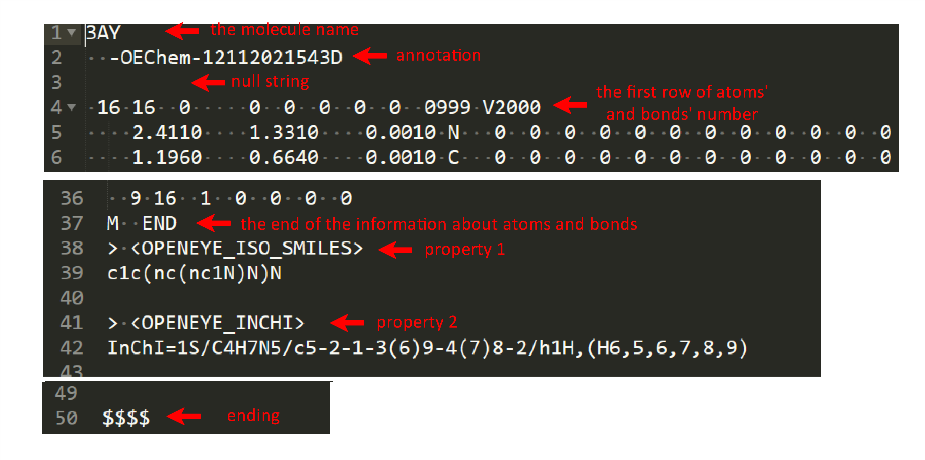
Small molecules should be upload as sdf files, such as ‘3AY_ideal.sdf’, different from RNA and protein. SDF is one of a family of chemical-data file formats developed by MDL. It is intended especially for structural information, starting with the molecule name and ending with four dollar signs (\$\$\$\$). In addition, other requirements are consistent with the above.

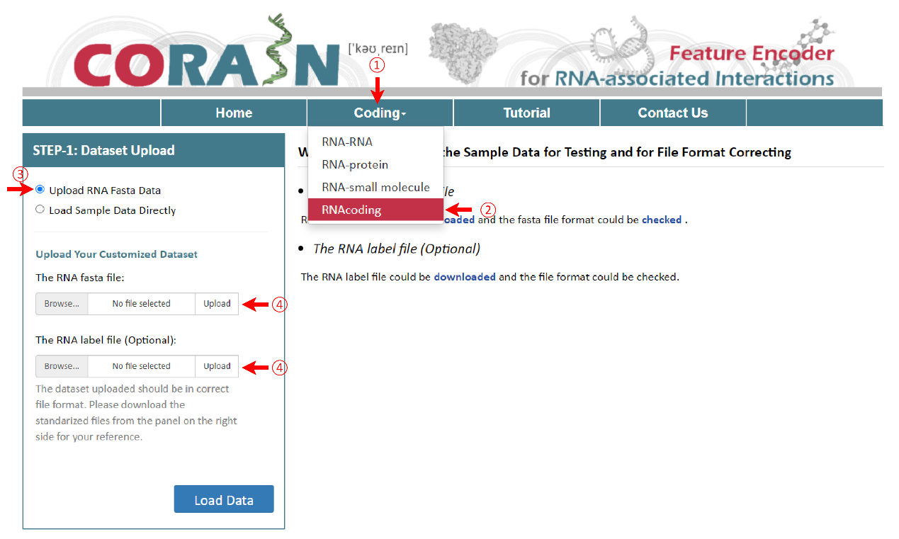
To get the encoding results of RNA, RNA fasta file and RNA label file are needed for further analysis. The RNA file format is same for the other three pages, such as ‘sampleData-RNA.fasta’. There are two columns in the RNA label file, sample name and class of samples. Their names are provided as "sequence ID" and "label". As well, the RNA label file must be csv format and the name of file and the last column can’t be changed.

Codon is a group of nucleotide triplets which specifies a single amino acid. It’s the set of rules used to construct genetic information. Codons are important indicators for transcripts coding into proteins (Shuai Liu, et al. Genes (Basel). 10: 672, 2019). Codon characteristics are fundamental sequence features and closely related to RNA coding potential.

Fickett score (FickS) is a simple linguistic feature that distinguishes protein-coding RNA (pcRNA) and non-coding RNA (ncRNA) according to the combinational effect of nucleotide composition and codon usage bias, first proposed by Fickett (J W Fickett, et al. Nucleic Acids Res. 10: 5303-18, 1982). It’s for RNA coding potential assessing independent of the ORF, and when the length of the test RNA region is ≥200nt, Fickett score alone can achieve 94% sensitivity and 97% specificity (Liguo Wang, et al. Nucleic Acids Res. 41: e74, 2013).
Calculation:
Fickett score is obtained by computing four position values and four composition values (base content) related coding potential from the transcript.
Position value reflects the degree to which each base is favored in one codon position versus another. For example, position value of A(A_position):

\[ A_1=\text{Number of As in position 0,3,6,…,3n} \]

\[ A_2=\text{Number of As in position 1,4,7,…,3n+1} \]

\[ A_3=\text{Number of As in position 0,3,6,…,3n+2} \]

$$ A_{position}=\frac{\max{(A_1,A_2,A_3)}}{\min{(A_1,A_2,A_3)}+1} $$ Position value of T_position, C_position, G_position are determined in the same way.
Composition values (base content) of each base (A_content, T_content, C_content, G_content) is easy to calculate.
Then these eight values can be converted into a probabilities (p) of coding table, which quantified from coding potential of real sequences of known function by Fickett (J W Fickett, et al. Nucleic Acids Res. 10: 5303-18, 1982).

Table 2 Characteristic Parameters of Coding and Noncoding Sequence

Position Parameter	Probability of Coding
	A	C	G	T
0.0~1.1	0.22	0.23	0.08	0.09
1.1~1.2	0.30	0.30	0.08	0.09
1.2~1.3	0.34	0.33	0.16	0.20
1.3~1.4	0.45	0.51	0.27	0.54
1.4~1.5	0.68	0.48	0.48	0.44
1.5~1.6	0.58	0.66	0.53	0.69
1.6~1.7	0.93	0.81	0.64	0.68
1.7~1.8	0.84	0.70	0.74	0.91
1.8~1.9	0.68	0.70	0.88	0.97
1.9~2.0+	0.94	0.80	0.90	0.97
Content Parameter	Probability of Coding
	A	C	G	T
0.0~0.17	0.21	0.31	0.29	0.58
0.17~0.19	0.81	0.39	0.33	0.51
0.19~0.21	0.65	0.44	0.41	0.69
0.21~0.23	0.67	0.43	0.41	0.56
0.23~0.25	0.49	0.59	0.73	0.75
0.25~0.27	0.62	0.59	0.64	0.55
0.27~0.29	0.55	0.64	0.64	0.40
0.29~0.31	0.44	0.51	0.47	0.39
0.31~0.33	0.49	0.64	0.54	0.24
0.33~0.99	0.28	0.82	0.40	0.28

Then Each probability is multiplied by a weight $w$ for the respective base, where the value of $w$ reflects the percentage of each parameter alone successfully predictions for the sequence of known function, also reported by Fickett (J W Fickett, et al. Nucleic Acids Res. 10: 5303-18, 1982) in weights $w$ of parameters table.

Table 3 Weight to be Given to the Individual Parameters

Methods	Position	Cotent
A	0.26	0.11
C	0.18	0.12
G	0.31	0.15
T	0.33	0.14

Finally, the Fickett score is calculated as follows:

\[ \text{Fickett Score}=\sum_{i=1}^8p_iw_i \]

A stop codon signals the termination of the current protein translation process (Martin Buncek, et al. Biologia Plantarum. 45:50-50, 2002).
Under standard conditions, there are three kinds of stop codons: UAG called amber, UGA called opal (sometimes also called umber), and UAA called ochre. While the start codon alone is not sufficient to begin the translation, usually need nearby sequences or initiation factors, stop codons alone are sufficient to initiate termination (Christian Touriol, et al. Biol Cell. 95:169-78, 2003). So it’s an important feature for RNA encoding.
Here we consider four types of STOP Codon-related Features.

Open reading frame (ORF) is a continuous stretch of codons, begins with a start codon (for RNA, usually AUG) and ends at a stop codon (for RNA, usually UAA, UAG or UGA), which has the ability to be translated.
The start-stop definition of an ORF only applies to mature mRNAs, not genomic DNA, since introns may contain stop codons and/or cause shifts between reading frames. Such an ORF corresponds to parts of a gene rather than the complete gene.
Since DNA/RNA is interpreted in groups of three-nucleotide codons, a DNA/RNA strand has three distinct reading frames. Meanwhile, the double helix of a DNA has two anti-parallel strands. With the two strands having three reading frames each, there are six possible frame translations for one DNA (W R Pearson, et al. Genomics. 46: 24-36, 1997).
Cheng Yang et al (Cheng Yang, et al. Bioinformatics. 34: 3825-3834, 2018) concluded that Open reading frame (ORF) is one of the most widely used and fundamental criteria to evaluate the coding potential of a sequence and distinguish an lncRNA from a coding transcript.

It’s reported that pcRNAs often contain longer ORFs than ncRNAs, and long ORFs are unlikely to be observed by random chance in ncRNAs, thus long ORFs are often one of the ideal and fundamental evidences to initially identify candidate protein-coding regions (Sen Yang, et al. Front Genet. doi: 10.3389/fgene.2020.00090. eCollection 2020, 2020; Jinfeng Liu, et al. PLoS Genet. 2: e29, 2006). ORF length as a feature is frugal, but it has high concordance with more sophisticated discrimination methods and remains the primary criterion in almost all coding-potential prediction methods (G S Zubenko, et al. J Neuropathol Exp Neurol. 49: 206-14, 1990; Liguo Wang, et al. Nucleic Acids Res. 41: e74, 2013; Lei Kong, et al. Nucleic Acids Res. 35: W345-9, 2007).
Here, not only restrict to ORF length, we consult to CPPred (Xiaoxue Tong, et al. Nucleic Acids Res. 47: e43, 2019) and introduce other ORF-based descriptions. For start codon setting, although the use of non-AUG has been constantly described (Nicholas T Ingolia, et al. Cell. 147: 789-802, 2011; Yafeng Zhu, et al. Nat Commun. 9: 903, 2018), AUG is still selected.
We use five types of Open Reading Frame Features (ORFF):

The entropy density profile (EDP) model is a global statistical description for a nucleotide sequence. It employs a Shannon's artificial linguistic description for a nucleotide sequence of finite length like an ORF or a transcript (Yongchu Liu, et al. BMC Bioinformatics. 14 Suppl 5(Suppl 5):S12, 2013).The EDP model has been proved to be successful and validates the hypothesis that the pcRNAs distribute separately from the ncRNAs in the EDP phase space, which may be caused by different selection pressures during the evolution (Huaiqiu Zhu, et al. BMC Bioinformatics. 8: 97, 2007).
Calculation:
Here, we employ EDP model on ORFs identified from input sequence. For the EDP based on k-mer frequency, we preset k-mer as a 3-mer (codon). And the EDP {si} of an ORF is defined as:

\[ s_i=-\frac{1}{H}c_i\log c_i \]

where $c_i$ is the abundance of the ith codon obtained by counting the number of it in the ORF sequence divided by the total number of codons, $i=1,2,\ldots,61$ represents the index of the 61 codons (excluding 3 stop codons), and $H=-\sum_{i=1}^{61}c_i\log c_i$ is the Shannon entropy.
Finally, we transform these s_i of 61 codons into eigenvalues of twenty corresponding native amino acids, and respectively named as:

Some biologically important oligomers (such as Hexamers) consist of many important macromolecules. For instance, hemoglobin is a protein tetramer. An oligomer of amino acids is called an oligopeptide. An oligonucleotide is a short single-stranded fragment of nucleic acid such as DNA or RNA. Many researches (J M Claverie, et al. Nucleic Acids Res. 14: 179-96, 1986; J M Claverie, et al. Methods Enzymol. 183: 237-52, 1990), revealed that some model for hexamers measure in frames can reflect to sequences differences (J W Fickett, et al. Nucleic Acids Res. 20: 6441-50, 1992).
Hexamer score on ORF (ORFHS), which means Hexamer usage bias on ORF. Hexamer usage bias (Hexamer score) is an essential feature because of the dependence between adjacent amino acids in pseudo proteins. Hexamer score is calculated based on in-frame hexamer frequency of protein-coding and non-coding RNA (J W Fickett, et al. Nucleic Acids Res. 20: 6441-50, 1992).
Calculation:
Here we consult to CPAT (Liguo Wang, et al. Nucleic Acids Res. 41: e74, 2013) and NCResNet (Sen Yang, et al. Front Genet. doi: 10.3389/fgene.2020.00090. eCollection 2020, 2020).CPAT used a log-likelihood ratio to measure differential hexamer usage between coding and noncoding sequences. For a given sequence, we identify its ORF and calculated the probability under the model of pcRNA and ncRNA trained by CPAT, and then we took the logarithm of the ratio of these probabilities as the score of coding potential. We used $F(H_i)(i=0,1,\ldots,4^6-1)$ and$F'(H_i)(i=0,1,\ldots,4^6-1)$to represent in-frame hexamer frequency. For a given hexamer sequence $S=H_1,H_2,…,H_m$

\[ \text{Hexamer Score}=\frac{1}{m}\sum_{i=1}^{m}\log(\frac{F(H_i)}{F'(H_i)}) \]

Hexamer score determines the relative degree of hexamer usage bias in a particular sequence. Positive values indicate a coding sequence, whereas negative values indicate a noncoding sequence (Shuai Liu, et al. Genes (Basel). 10: 672, 2019).
However, Hexamer score only computes the average hexamer frequencies of the training data sets. For any unknown sequence, the hexamer patterns are scanned, but their frequencies are abandoned. The main idea underlying the proposed measurements is to estimate the unevaluated sequence is ‘close to’ ncRNA or pcRNA. Here, we consult to LncFinder (Siyu Han, et al. Brief Bioinform. 20: 2009-2027, 2019) and propose the following two new measurements to quantify the usage bias of hexamer on ORF, Euclidean distance and Logarithm distance, and get six eigenvalues:Hexamer logarithm distance to lncRNA ORF (ORLoL); Hexamer logarithm distance to pcRNA ORF (ORLoP); Hexamer logarithm distance ORF ratio (ORLoR); Hexamer euclidean distance to lncRNA ORF (OREuL); Hexamer euclidean distance to pcRNA ORF (OREuP); Hexamer euclidean distance ORF ratio (OREuR).
Calculation:

\[ ORLoL=\frac{1}{n}\sum{In\frac{freq.seq(i)}{freq.lnc(i)}},i=1,2,3,\ldots,4^k \]

\[ ORLoP=\frac{1}{n}\sum{In\frac{freq.seq(i)}{freq.pc(i)}},i=1,2,3,\ldots,4^k \]

\[ ORLoR=\frac{\log{Dist.LNC}}{\log{Dist.PC}} \]

\[ OREuL=\sqrt{\sum(freq.seq(i)-freq.lnc(i))^2},i=1,2,3,\ldots,4^k \]

\[ OREuP=\sqrt{\sum(freq.seq(i)-freq.pct(i))^2},i=1,2,3,\ldots,4^k \]

\[ OREuR=\frac{EucDist.LNC}{EucDist.PC} \]

where freq.seq are the k-adjoining base(s) frequencies of one unevaluated sequence; freq.lnc denotes the average frequencies of lncRNAs’ k-adjoining base(s) ; freq.pct denotes the average frequencies of pcRNAs’ k-adjoining base(s); i denotes the different types of k-adjoining base(s), and n is the total number of the k-adjoining base(s) in one sequence. Based on first two equations, OREuL and logORLoP can be computed. EucDist.PC and logDist.PC can be obtained similarly.

As we all know, there are four kinds of nitrogenous bases, Adenine (A), Guanine (G), Cytosine (C), and Thymine (T), which bind to sugar and phosphate to form four kinds of nucleotides for DNA. In its double-stranded helical structure, the bases on one strand must pair up with bases on another strand, Adenine pair up with Thymine (A/T or T/A) and Cytosine pair up with Guanine (C/G or G/C). This principle of arrangement is called Complementary Base Pairing (James D Watson, et al. Clin Orthop Relat Res. 462: 3-5, 2007). For RNAs, Uracil (U) equals to Thymine (T).
Quantitatively, each Guanine/Cytosine (G/C) base pair is held by three hydrogen bonds, while Adenine/Thymine (A/T) and Adenine/ Uracil (A/U) base pairs are held by two hydrogen bonds. For a long nucleotide sequence, interactions of base stacking have obvious influence on molecular stability (Peter Yakovchuk, et al. Nucleic Acids Res. 34: 564-74, 2006). So, it’s easy to understand that nucleic acid with low GC content (the percentage of nitrogenous bases guanine and cytosine on a nucleic acid molecule) is less stable than nucleic acid with high GC-content.
For RNAs, Pozzoli U et al. pointed that the length of the coding sequence (CDS) is directly proportional to higher GC content (Uberto Pozzoli, et al. BMC Evol Biol. 27; 8:99, 2008). And it has been pointed the fact that the stop codon has a bias towards A and T nucleotides, and, thus, the shorter the sequence the higher the AT content (J D Wuitschick, et al. J Eukaryot Microbiol. 46: 239-47, 1999). Also, it has been pointed that there is a strong correlation between the GC-content of structural RNAs and the optimal growth of prokaryotes at higher temperatures, such as ribosomal RNA, transfer RNA, and many other non-coding RNAs (L D Hurst, et al. Proc Biol Sci. 268:493-7, 2001). Shuai Liu et al. pointed that GC content may play an important role in the prediction of RNA coding potential (Shuai Liu, et al. Genes (Basel). 10: 672, 2019).
Calculation
The percentage of G and C on nucleotide strand can be used to calculate the GC content of the sequence and GC content in the first, second and third position of codons.

\[ \frac{G+C}{A+T+G+C}\times100\% \]

The variance of them among three reading frames can also be considered.

Transcription is the first of several steps of DNA based gene expression. A particular segment of DNA is translated into a complementary, antiparallel RNA strand called primary transcript by the RNA polymerase. The primary transcripts are further modified by several processes, including the 5' cap, 3'-polyadenylation, and alternative splicing, to yield various mature RNA products (so called transcripts) such as mRNAs, tRNAs, rRNAs and so on. Particularly, alternative splicing directly contributes to the diversity of mRNA found in cells.
Different kinds of transcripts have characteristics in different fields, which can be descriptions for RNA features.

Untranslated region (UTR) refers to two sections, on each side of a coding sequence (CDS) on a strand of mRNA. If it is on the 5' side, it is called the 5' UTR (or leader sequence); if it is on the 3' side, it is called the 3' UTR (or trailer sequence).5' and 3' UTRs usually not translated into protein, but uORFs located within the 5' UTR can be translated into peptides (Cristina Vilela, et al. Mol Microbiol. 49: 859-67, 2003).The 5' UTR contains a ribosome-recognizing-sequence, which allows the ribosome to bind and initiate translation. The 3' UTR usually subsequently follow the stop codon, plays an important role in translation termination and post-transcriptional modification (Lucy W Barrett, et al. Cell Mol Life Sci. 69: 3613-34, 2012). Introns are not untranslated regions, because they are spliced out in the process of RNA splicing and not included in the mature mRNA molecule that will undergo translation.
It has been known that the UTR of mRNA is involved in many regulatory aspects of gene expression in eukaryotic organisms (Shuai Liu , et al. Genes (Basel). 10:672, 2019), meanwhile, it has several noteworthy characteristics, for example, 3’ UTRs are generally much longer than 5’ UTRs (Cheng Yang , et al. Bioinformatics. 34: 3825-3834, 2018).
The features of UTR indicate the coding potential of transcript, here we consult to LncADeep (Cheng Yang , et al. Bioinformatics. 34: 3825-3834, 2018), use four of Untranslated region related Features:

K-mer means dividing a sequence into substrings containing k bases. If the length of sequence is L and the length of k-mer is k, the number of k-mers generated is L-k+1, and the number of kinds of k-mers generated is 4^k.
K-mer is a simple approach to represent nucleotide sequences, which are represented as the occurrence frequencies of k neighboring nucleic acids. This approach has been successfully applied to human gene regulatory sequence prediction (William Stafford Noble, et al. Bioinformatics. Suppl 1: i338-43, 2005), enhancer identification (, Dongwon Lee, et al. Genome Res. 21: 2167-80, 2011), etc.
Here, we consult to Jessime M Kirk et al.’s research (Jessime M Kirk, et al. Nat Genet. 50: 1474-1482, 2018) , and count each kind of mer as a 4^kD feature (preset k=3 (codon)),respectively named as:

CTD encoding is a computing strategy for sequence representation such as nucleotide sequences, amino acid sequence and so on (L Y Han, et al. Nucleic Acids Res. 32:6437-44, 2004). CTD features (composition, transition, and distribution) captured can convert a sequence into a digital feature vector, based on the characteristics including basic sequence information, physicochemical properties or other appropriate features (Xiaoxue Tong, et al. Nucleic Acids Res. 47: e43, 2019; Feng Zhu, et al. J Pharmacol Exp Ther. 330:304-15, 2009).
Global transcript sequence descriptors denote the global transcript sequence descriptions using CTD encoding, including nucleotide composition, nucleotide transition and nucleotide distribution. The first descriptor nucleotide composition describes the percent composition of each nucleotide in a transcript sequence. The second descriptor nucleotide transition describes the percent frequency with conversion of four nucleotides between adjacent positions. The third descriptor nucleotide distribution describes five relative positions along the transcript sequence of each nucleotide, calculated with the 0 (first one), 25%, 50%, 75% and 100% (last one) (Xiaoxue Tong, et al. Nucleic Acids Res. 47: e43, 2019).
Take one nucleotide sequence as an example, ACTTGCAGCCCCCCGCCTGTCCCGAGCCGCGCGGGCGCCAGCTCAGTTTGTCCGCGGCGG, with 5 adenines (As), 9 thymines (Ts), 20 guanines (Gs) and 26 cytidines (Cs) (Xiaoxue Tong, et al. Nucleic Acids Res. 47: e43, 2019).
First descriptor composition C are four features respectively:
$$Composition of A (ComRA) = 5/60 = 0.083;$$ $$Composition of T (ComRT) = 9/60 = 0.15;$$ $$Composition of G (ComRG) = 20/60 = 0.33;$$ $$Composition of C (ComRC) = 26/60 = 0.43$$ Second descriptor transition T are six features respectively, there is zero transition between A and T, five transitions between A and G, four transitions between A and C, five transitions between T and G, six transitions between T and C and twenty transitions between G and C: $$Transition between A and T (TraAT) = 0/59 = 0.00;$$ $$Transition between A and G (TraAG) = 5/59 = 0.085;$$ $$Transition between A and C (TraAC) = 4/59 = 0.068;$$ $$Transition between T and G (TraTG) = 5/59 = 0.085;$$ $$Transition between T and C (TraTC) = 6/59 = 0.10;$$ $$Transition between G and C (TraGC) = 20/59 = 0.34.$$ Third descriptor distribution D are 20 features respectively, The first, 25%, 50%, 75% and 100% of As are located within 1, 1, 25, 40 and 45 residues: $$Distribution of 0.00A (DPRA0) = 1/60 = 0.017;$$ $$Distribution of 0.25A (DPRA1) = 1/60 = 0.017;$$ $$Distribution of 0.50A (DPRA2) = 25/60 = 0.42;$$ $$Distribution of 0.75A (DPRA3) = 40/60 = 0.67;$$ $$Distribution of 1.00A (DPRA4) = 45/60 = 0.75.$$ Likewise, the D descriptors for Ts, Gs and Cs are: $$Distribution of 0.00T (DPRT0) = 0.05;$$ $$Distribution of 0.25T (DPRT1) = 0.067;$$ $$Distribution of 0.50T (DPRT2) = 0.72;$$ $$Distribution of 0.75T (DPRT3) = 0.80;$$ $$Distribution of 1.00T (DPRT4) = 0.85;$$ $$Distribution of 0.00G (DPRG0) = 0.083;$$ $$Distribution of 0.25G (DPRG1) = 0.40;$$ $$Distribution of 0.50G (DPRG2) = 0.57;$$ $$Distribution of 0.75G (DPRG3) = 0.83;$$ $$Distribution of 1.00G (DPRG4) = 1.00;$$ $$Distribution of 0.00C (DPRC0) = 0.033;$$ $$Distribution of 0.25C (DPRC1) = 0.22;$$ $$Distribution of 0.50C (DPRC2) = 0.38;$$ $$Distribution of 0.75C (DPRC3) = 0.65;$$ $$Distribution of 1.00C (DPRC4) = 0.97;$$

Similar to the Entropy density profiles on ORF, we also consider Entropy density profiles on transcript, which can be calculated by analogy.

Similar to the Measurement of Hexamer on ORF, we also consider Measurement of Hexamer on transcript, which can be calculated by analogy.
Hexamer score on transcript (TraHS), which means Hexamer usage bias on transcript.
Euclidean distance and Logarithm distance quantification of Hexamer score on transcript:
Hexamer logarithm distance to lncRNA transcript (TrLoL); Hexamer logarithm distance to pcRNA transcript (TrLoP); Hexamer logarithm distance transcript ratio (TrLoR); Hexamer euclidean distance to lncRNA transcript (TrEuL); Hexamer euclidean distance to pcRNA transcript (TrEuP); Hexamer euclidean distance transcript ratio (TrEuR).

One-hot encoding is a binary vector with the matching character entry being 1s and 0s(Jack Lanchantin, et al. Pac Symp Biocomput. 22:254-265, 2017).
Sequence-based one-hot encoding (SeqOH). Here, the input nucleotide sequence is represented as a one-hot representation encoded into a binary matrix, whose columns correspond to the presence of A, C, G, T and N (for unconfirmed base) (Babak Alipanahi, et al. Nat Biotechnol. 33:831-8, 2015; Jian Zhou, et al. Nat Methods. 12:931-4, 2015). Given a sequence with n nucleotides and sequence motif detector with defined size m, the binary matrix M for this sequence is represented as follows(Xiaoyong Pan, et al. BMC Genomics. 19:511, 2018).
$$ M_{i,j} \begin{cases} 0.25\ \ \ if\ s_{i-m+1}=N\ or\ i\lt m\ or\ i\gt n-m\\\ 1\ \ \ if\ j=A,s_{i-m+1}\ is\ (A)\\\ 1\ \ \ if\ j=C,s_{i-m+1}\ is\ (C)\\\ 1\ \ \ if\ j=G,s_{i-m+1}\ is\ (G)\\\ 1\ \ \ if\ j=U,s_{i-m+1}\ is\ (U)\\\ 0\ \ \ otherwise \end{cases} $$ where $i$ is the index of the nucleotide, $j$ is the index of the column corresponding to $A,C,G,T$.

Word2vec is a word vector generation tool based on unsupervised learning, using Wikipedia as corpus (Moe Matsuki, et al. Nat Methods. 12:931-4, 2015).The advantages of using word2vec is that (a) the word embedding can be automatically generated, (b) no identical vectors are created, and (c) the word embedding is adequate as semantic embedding space (Moe Matsuki, et al. Nat Methods. 12:931-4, 2015).
Sequence-based word2vec embeddings (SeqWE). Here, for a nucleotide sequence, each nucleotide has interconnections and Word2vec embedding has the opportunity to abstract such sequence features, reflecting the relationship between each word (Moe Matsuki, et al. Nat Methods. 12:931-4, 2015).
Semantic vectors generated from word2vec have been comprehensively used in image recognition (Moe Matsuki, et al. Nat Methods. 12:931-4, 2015), and has been generally used in RNA and protein sequence representation for lncRNA-protein interactions prediction (Hai-Cheng Yi, et al. Comput Struct Biotechnol J. 18:20-26, 2019).

NcRNAs cannot be translated to produce true proteins, so it’s easy to understand that the pseudo protein translated by ncRNA doesn’t have true protein sequence and physicochemical features (Peter J A Cock, et al. Front Genet. 11: 90, 2020). Pseudo protein related physicochemical features are reliable for ncRNA description.
Based on the understanding above, we select and calculate five related protein characters as features by Biopython (Sen Yang, et al. Bioinformatics. 25: 1422-3, 2009):

Here, we consult to Bin Liu et al.’s research (Bin Liu, et al. Bioinformatics. 31: 1307-9, 2015) and use two kinds of model, Autocorrelation and pseudo nucleic acid composition, to formulate transcript with dinucleotide physicochemical features. It’s calculated by their repDNA python package. The Table 12 include the 38 dinucleotide physicochemical features considered in the calculation below (Bin Liu, et al. Bioinformatics. 31: 1307-9, 2015).

Autocorrelation is a multivariate modeling tools, which can transform different length of nucleotide sequences into fixed-length vectors by measuring the correlation between any two properties. Autocorrelation results in two kinds of variables: autocorrelation (AC) between the same property, and cross-covariance (CC) between two different properties (Bin Liu, et al. Bioinformatics. 31: 1307-9, 2015).
Dinucleotide auto covariance (Bin Liu, et al. Bioinformatics. 31: 1307-9, 2015).
Dinucleotide auto covariance (DAC) incorporates the correlation of the same property between two dinucleotides.
Suppose the nucleotide sequence D with L nucleic acid residues:

\[ D=R_1R_2R_3R_4R_5R_6R_7\ldots R_L \]

$R_1$ represents the nucleic acid residue at the sequence position 1, $R_2$ represents the nucleic acid residue at position 2 and so forth.
The DAC measures the correlation of the same physicochemical index between two dinucleotides separated by a distance of lag along the sequence, which can be calculated as:

\[ DAC(u,lag)=\sum_{i=1}^{L-lag-1} (P_u(R_iR_{i+1})-\overline{P_u})(P_u(R_{i+lag}R_{i+lag+1})-\overline{P_u})/(L-lag-1) \]

where $u$ is a physicochemical index considered that are listed in the Table 12, $L$ is the length of the sequence, $P_u(R_iR_{i+1})$ means the numerical value of the physicochemical index $u$ for the dinucleotide $R_iR_{i+1}$ at position $i$, $\overline{P_u}$ is the average value for physicochemical index $u$ along the whole sequence:

\[ \overline{P_u}=\sum_{j=1}^{L-1}P_u (R_j R_{j+1} ) /(L-1) \]

In such a way, there are N*LAG of DAC feature values, where N is the number of physicochemical indices and LAG is the maximum of lag (lag=1,2,…,LAG). Here, N = 38 and LAG is preset to 2. Thus, the feature vector is Dinucleotide auto covariance of lag1 on BST (ABST1) ~ Dinucleotide auto covariance of lag2 on RIS (ARIS2), 78 values totally. The complete short names are summarized in the following Table 13.
This DAC approach is similar as the approach used for protein fold recognition (Qiwen Dong, et al. Bioinformatics. 25: 2655-62, 2009).
Dinucleotide-based cross covariance (Bin Liu, et al. Bioinformatics. 31:1307-9, 2015)
Given a nucleotide sequence D (analogy to above), the DCC measures the correlation of two different physicochemical indices between two dinucleotides separated by lag nucleic acids along the sequence, which can be calculated by:

\[ DCC(u_1,u_2,lag)=\sum_{i=1}^{L-lag-1}(P_{u_1}(R_iR_{i+1})-\overline{P_{u_1}})(P_{u_2}(R_{i+lag}R_{i+lag+1})-\overline{P_{u_2}})/(L-lag-1)) \]

where $u_1$, $u_2$ are two different physicochemical indices considered that are listed in the Table 12, $L$ is the length of the sequence, $P_{u_1}(R_iR_{i+1})$($P_{u_2}(R_iR_{i+1})$) is the numerical value of the physicochemical index $u_1$ ($u_2$) for the dinucleotide $R_iR_{i+1}$ at position $i$, $\overline{P_{u_1}}$ ($\overline{P_{u_2}}$) is the average value for physicochemical index value $u_1$, $u_2$ along the whole sequence:

\[ \overline{P_u}=\sum_{j=1}^{L-1}P_u (R_j R_{j+1} ) /(L-1) \]

In such a way, the length of the DCC feature vector is N*(N-1)*LAG, where N is the number of physicochemical indices and LAG is the maximum of $lag$ ($lag$=1,2,…,LAG).
Here, we pick out N=6 representative physicochemical features for DCC calculation, including PID, BDS, ETI, SKE, WCI, SLI, PID, BDS, ETI, SKE, WCI, SLI, and LAG is preset to 2. Thus, the feature vector is Cross covariance of lag1 on PID-BDS (CC101) ~ Cross covariance of lag2 on SLI-WCI (CC230), 60 values totally.
This DCC approach is similar as the approach used for protein fold recognition (Qiwen Dong, et al. Bioinformatics. 25: 2655-62, 2009).

Pseudo nucleic acid composition (PseNAC) is a kind of powerful approaches to represent the nucleotide sequence considering both local sequence-order information and long range or global sequence-order effects. Concretely here, as for Pseudo dinucleotide composition (PseDNC), it incorporates the contiguous local sequence-order information and the global sequence-order information into the feature vector of the nucleotide sequence. Here are two types of PseNAC considered (Bin Liu, et al. Bioinformatics. 31: 1307-9, 2015).
Parallel correlation pseudo dinucleotide composition (PC-PseDNC)
Parallel correlation PseDN composition (PC-PseDNC) can be calculated not only based on 38 built-in physiochemical properties (Table 13), but also other indices defined by users.
Given a nucleotide sequence D, the PC-PseDNC feature vector of D is defined:

\[ D=[d_1 d_2 \ldots d_{16}d_{16+1} \ldots d_{16+λ}]^T \]

where:

\[ d_k= \begin{cases} f_k\over\sum_{i=1}^{16}f_i +w\sum_{j+1}^\lambda \theta_j& (1\leq k \leq 16)\\\\ w\theta_{k-16}\over\sum_{i=1}^{16}f_i+w\sum_{j=1}^\lambda\theta_j& (17\leq k\leq16+\lambda) \end{cases} \]

where $f_k$ ($k$=1,2,⋯,16) is the normalized occurrence frequency of dinucleotide in the sequence; the parameter λ is an integer, representing the highest counted rank (or tier) of the correlation along a sequence; $w$ is the weight factor ranged from 0 to 1; $θ_j$ ($j$=1,2,⋯,λ) is called the j-tier correlation factor that reflects the sequence-order correlation between all the most contiguous dinucleotides along a sequence, which is defined:

\[ (\lambda\lt L) \begin{cases} \theta_1=\frac{1}{L-2}\sum_{i=1}^{L-2}\theta(R_iR_{i+1},R_{i+1}R_{i+2})\\\ \theta_2=\frac{1}{L-3}\sum_{i=1}^{L-3}\theta(R_iR_{i+1},R_{i+2}R_{i+3})\\\ \theta_3=\frac{1}{L-4}\sum_{i=1}^{L-4}\theta(R_iR_{i+1},R_{i+3}R_{i+4})\\\ \cdots\\\ \theta_\lambda=\frac{1}{L-1-\lambda}\sum_{i=1}^{L-1-\lambda}\theta(R_iR_{i+1},R_{i+\lambda}R_{i+1+\lambda}) \end{cases} \]

where the correlation function is given by

\[ \theta(R_iR_{i+1},R_{j}R_{j+1})=\frac{1}{\mu}\sum_{u=1}^\mu[P_u(R_iR_{i+1})-P_u(R_{j}R_{j+1})]^2 \]

where $μ$ is the number of physicochemical indices considered that are listed in the Table 12; $P_u(R_iR_{i+1})$ ($P_u(R_jR_{j+1})$) represents the numerical value of the $u$-th ($u$=1,2,⋯,μ) physicochemical index for the dinucleotide $R_iR_{i+1}$ ($R_jR_{j+1}$) at position $i$ and $j$, respectively.
Here, λ is preset to 2. Thus, the feature vector (d_ks) is Parallel correlation PseDN composition of AA (PCDAA) ~ Parallel correlation PseDN composition of GG (PCDGG), & Parallel correlation PseDN composition of lamda1 (PCDl1) ~ Parallel correlation PseDN composition of lamda2 (PCDl2), 18 values totally. The complete short names are summarized in the following Table 14.
For more information of PC-PseDNC approach, you can refer to (Wei Chen, et al. Anal Biochem. 456: 53-60, 2014).
Series correlation PseDN composition:
Series correlation PseDN composition (SC-PseDNC) is a variant of PC-PseDNC. Combining dinucleotide composition and global sequence-order effects by series correlation.
Given a nucleotide sequence D, the SC-PseDNC feature vector of D is defined:

\[ D=[d_1d_2\ldots d_{16}d_{16+1}\ldots d_{16+\lambda}d_{16+\lambda+1}\ldots d_{16+\lambda\Lambda} ]^T \]

where

\[ d_k=\begin{cases} \frac{f_k}{\sum_{i=1}^{16}f_i+w\sum_{j=1}^\lambda\theta_j}&(1\leq k\leq 16)\\\ \frac{w\theta_{k-16}}{\sum_{i=1}^{16}f_i+w\sum_{j=1}^{\lambda\Lambda}\theta_j}&(17\leq k\leq16+\lambda\Lambda) \end{cases} \]

where $f_k$ ($k$=1,2,⋯,16) is the normalized occurrence frequency of dinucleotide in the sequence; the parameter λ is an integer, representing the highest counted rank (or tier) of the correlation along a sequence; $w$ is the weight factor ranged from 0 to 1; Λ is the number of physicochemical indices; $θ_j$ ($j$=1,2,⋯,λ) is called the j-tier correlation factor that reflects the sequence-order correlation between all the most contiguous dinucleotides along a sequence, which is defined:

\[ (\lambda\lt L-2) \begin{cases} \theta_1=\frac{1}{L-3}\sum_{i=1}^{L-3}\it J_{i.i+1}^1\\\ \theta_2=\frac{1}{L-3}\sum_{i=1}^{L-3}\it J_{i.i+1}^2\\\ \ldots\\\ \theta_\Lambda=\frac{1}{L-3}\sum_{i=1}^{L-3}\it J_{i.i+1}^\Lambda\\\ \cdots\\\ \theta_{\lambda\Lambda-1}=\frac{1}{L-\lambda-2}\sum_{i=1}^{L-\lambda-2}\it J_{i.i+\lambda}^{\Lambda-1}\\\ \theta_{\lambda\Lambda}=\frac{1}{L-\lambda-2}\sum_{i=1}^{L-\lambda-2}\it J_{i.i+\lambda}^{\Lambda} \end{cases} \]

The correlation function is given by:

\[ \begin{cases} J_{i,i+m}^\zeta=P_u(R_iR_{i+1})\cdot P_u(R_{i+m}R_{i+m+1})\\\ \zeta=1,2,\cdots,\Lambda;m=1,2,\cdots,\lambda;i=1,2,\cdots,L-\lambda-2 \end{cases} \]

where $μ$ is the number of total physiochemical indices (Table 12); $P_u(R_iR_{i+1})$ ($P_u(R_jR_{j+1})$) represents the numerical value of the $u$-th ($u$=1,2,⋯,μ) physiochemical index for the dinucleotide $R_iR_{i+1}$ ($R_jR_{j+1}$) at position $i$($j$).
Here, we pick out Λ=6 representative physicochemical features for SC-PseDNC calculation, including PID, BDS, ETI, SKE, WCI, SLI, PID, BDS, ETI, SKE, WCI, SLI, λ is preset to 2. Thus, the feature vector (d_ks) is Series correlation PseDN composition of AA (SCDAA) ~ Series correlation PseDN composition of GG (SCDGG), & Series correlation PseDN composition of lamda1-PID (L1PID) ~ Series correlation PseDN composition of lamda2-SLI (L2SLI), 28 values totally. The complete short names are summarized in the following Table 15. For more information of the SC-PseDNC, please refer to (Wei Chen, et al. Anal Biochem. 456: 53-60, 2014).

Electron-ion interaction pseudopotential (EIIP), calculate the energy of delocalized electrons in amino acids and nucleotides (Siyu Han, et al. Brief Bioinform. 20: 2009–2027, 2019). For any DNA sequence, each nucleotide (A, C, G and T) owns and can be replaced by the following EIIP values: {A→0.1260; C→0.1340; G→0.0806; T→0.1335} (Dragutin Lalović, Veljko Veljković. Biosystems. 23: 311-316, 1990). It was primordially used to locate exons (Dragutin Lalović, Veljko Veljković. Biosystems. 23: 311-316, 1990). Compared with pI values, DNA EIIP values can be directly applied to RNA sequences, which can avoid the potential bias caused by the speculated translation process (Siyu Han, et al. Brief Bioinform. 20: 2009–2027, 2019).
EIIP-based spectrum embodies the physicochemical and 3-base periodicity properties of pcRNAs (A A Tsonis, et al. J Theor Biol. 151: 323-31, 1991; S Tiwari, et al. Comput Appl Biosci. 13: 263-270, 1997). It has been proved that features from this category can present robust results (Siyu Han, et al. Brief Bioinform. 20: 2009–2027, 2019).
Calculation:
We consult to LncFinder (Siyu Han, et al. Brief Bioinform. 20: 2009–2027, 2019) and let $X_e[n]$ be the EIIP indicator value at nth position of a sequence. Using Fast Fourier transform (FFT) on $X_e[n]$, a Sequence Power Spectrum of an RNA can be calculated by the following equation (Sen Yang, et al. Front Genet. 11: 90, 2020):

\[ X_e[k]=\sum_{n=0}^{N-1}X_e[n]e^{-j\frac{2\pi kn}{N}} \]

\[ S_e[k]=|X_e[k]|^2=|\sum_{n=0}^{N-1}X_e[n]e^{-j\frac{2\pi kn}{N}}|^2 \]

\[ (k=0,1,2,\ldots,N-1;\text{N is the sequence length}) \]

It has been reported that pcRNA has a different Power Spectrum distribution compared with ncRNAs. And generally, in the power spectrum of a pcRNA, a peak value will emerge in the thirds position but will not appear in ncRNA (Siyu Han, et al. Brief Bioinform. 20: 2009–2027, 2019).
Thus, based on the difference, here we can employ three physicochemical properties from Sequence Power Spectrum as features.
Electron-ion interaction pseudopotential signal peak (EipSP), which records the signal value of the third position (peak value):

\[ EipSP=S_e[\frac{N}{3}] \]

It has been noted that most of lncRNAs possess lower $S_e[\frac{N}{3}]$ by Han et al (Siyu Han, et al. Brief Bioinform. 20: 2009–2027, 2019).
Electron-ion interaction pseudopotential average power (EipAP), which records the averaging power of a sequence:

\[ EipAP=\frac{\sum_{k=0}^{N-1}S_e[k]}{N} \]

Electron-ion interaction pseudopotential signal/noise ratio (EiSNR), which is equal to EipSP divided by the EipAP:

\[ EiSNR=\frac{EipSP}{EipAP} \]

It has been noted that most of lncRNAs possess lower EipAP and EiSNR values by Han et al (Siyu Han, et al. Brief Bioinform. 20: 2009–2027, 2019).
In addition to three EIIP based sequence power spectrum features above, we sorted the sequence power spectrum in descending order to sample five position values, which are:
Electron-ion interaction pseudopotential spectrum 0 (EiPS0), corresponding to the minimum of sorted Power Spectrum values; Electron-ion interaction pseudopotential spectrum 0.25 (EiPS1), corresponding to the lower quartile value of sorted Power Spectrum values; Electron-ion interaction pseudopotential spectrum 0.5 (EiPS2), corresponding to the medium value of sorted Power Spectrum values; Electron-ion interaction pseudopotential spectrum 0.75 (EiPS3), corresponding to the upper quartile value of sorted Power Spectrum values; Electron-ion interaction pseudopotential spectrum 1 (EiPS4), corresponding to the maximum value of sorted Power Spectrum values (Siyu Han, et al. Brief Bioinform. 20: 2009–2027, 2019; Sen Yang, et al. Front Genet. 11: 90, 2020).
The ranges in the first group varies from the top 10 to top 100 of the sorted power spectrum, and the ranges are also from the top 10% to 100% of the sorted power spectrum. As the signals of mRNAs are generally stronger than those of lncRNAs, pcRNAs should tend to have higher values of these quantiles’ statistics than lncRNAs (Siyu Han, et al. Brief Bioinform. 20: 2009–2027, 2019).

In addition to calculation on basic sequence information in Global transcript sequence descriptors above (Xiaoxue Tong, et al. Nucleic Acids Res. 47:e43, 2019), here, we set 4 physicochemical characteristics for CTD encoding: Solubility lipoaffinity, Partition coefficient, Polarizability refractivity and Hydrogen bond related. Detailed information on how to construct this physicochemical CTD characteristics is provided in our previous studies (Feng Zhu, et al. J Pharmacol Exp Ther. 330:304-15, 2009).

According to the Solubility (mol/ml) at 25℃, calculated by PaDEL-descriptor(Chun Wei Yap, et al. J Comput Chem. 32:1466-74, 2011), we divide ACGT into two groups: A and B, as the Table 16 shows:

Then we encode the sequence using CTD computing strategy introduced above based on GroupA and GroupB. Eigenvalues are respectively named as:

According to the Lipoaffinity index, calculated by PaDEL-descriptor (Chun Wei Yap, et al. J Comput Chem. 32:1466-74, 2011), we divide ACGT into two groups: A and B, as the Table 18 shows:

Then we encode the sequence using CTD computing strategy introduced above based on GroupA and GroupB. Eigenvalues are respectively named as:

In addition to Global transcript sequence descriptors above and physicochemical CTD characteristics above(Xiaoxue Tong, et al. Nucleic Acids Res. 47: e43, 2019), here, we set 2 Structure-based characteristics for CTD encoding: Topological indice and Molecular fingerprint. Detailed information on how to construct this Structure-based CTD characteristics is provided in our previous studies.(Feng Zhu, et al. J Pharmacol Exp Ther. 330: 304-15, 2009).

According to the Molecular distance edge between all secondary carbons, calculated by PaDEL-descriptor(Chun Wei Yap, et al. J Comput Chem. 32: 1466-74, 2011), we divide ACGT into two groups: A and B, as the Table 30 shows:

According to the Molecular distance edge between all primary and secondary nitrogens, calculated by PaDEL-descriptor(Chun Wei Yap, et al. J Comput Chem. 32: 1466-74, 2011), we divide ACGT into two groups: A and B, as the Table 32 shows:

According to the Number of hydrogen atoms, calculated by PaDEL-descriptor(Chun Wei Yap, et al. J Comput Chem. 32: 1466-74, 2011), we divide ACGT into two groups: A and B, as the Table 34 shows:

According to the Number of quadruple bonds, calculated by PaDEL-descriptor(Chun Wei Yap, et al. J Comput Chem. 32: 1466-74, 2011), we divide ACGT into two groups: A and B, as the Table 36 shows:

According to the Count of atom-type E-State: -NH-, calculated by PaDEL-descriptor(Chun Wei Yap, et al. J Comput Chem. 32: 1466-74, 2011), we divide ACGT into two groups: A and B, as the Table 38 shows:

It’s reported that ncRNAs often have lack sequence conservation（Sen Yang, et al. Front Genet. 11: 90, 2020). Thus, RNA Secondary structure conservation is taken into consideration.

Secondary structural conservation (SecSC).Here, we calculate the eigenvalue by scanning the bin sequence against Rfam with the INFERNAL(Eric P Nawrocki, et al. Bioinformatics. 29: 2933-5, 2013) program (a binary score indicating the existence of a homologous structure in Rfam)(Long Hu, et al. Nucleic Acids Res. 45: e2, 2017).

It’s reported that although most lncRNAs are stable, mRNAs are usually more stable than lncRNAs(Hidenori Tani, et al. Methods Mol Biol. 1262: 305-20, 2015). The minimum free energy (MFE) is a basic structural outline index that evaluates the stability of the secondary structure of RNAs, which show that mRNAs generally tend to possess lower MFE.

In addition to this, we used a number of secondary structure-based features, in terms of the minimum free energy (MFE), paired bases and unpaired bases to form four features vector to represent the transcripts(Xiao-Nan Fan, et al. Mol Biosyst. 11: 892-7, 2015). These feature values can be given by the RNAfold program(Daniel M Blumenthal, et al. J Gen Intern Med. 30: 724-31, 2015).:

Secondary structural minimum free energy (SDMFE), which means the minimum free energy ($v_{MFE}$) of transcript;
Secondary structural average MFE (SAMFE), which means $\frac{v_{MFE}}{L}$, where $L$ is the length of transcript;
Secondary structural paired bases (SSDPB), which means the number of paired bases;
Secondary structural unpaired bases (SSDUB), which means the number of unpaired bases.

Siyu Han et al.(Siyu Han, et al. Brief Bioinform. 20: 2009-2027, 2019) first introduce a kind of multi-scale secondary structural information based self-design RNA sequence from three levels: stability, secondary structure elements (SSEs) combined with pairing condition and structure-nucleotide sequences, which is a special way for sequence representation.

Low-scale feature (stability): MFE is a basic structural outline displaying the stability of the RNA structure, Thus, MFE is selected as the low-scale feature.

Medium-scale feature (SSEs): Let $seq[n]$ be an RNA sequence with length $N$, and the nucleotides are denoted in lowercase $seq[n]\in\{a,c,g,u\}$;Let $SS[n]$ be the secondary structure sequence of $seq[n]$, and $SS[n]$ is defined using dot-bracket notation $(SS[n]\in\{\ .\ \ ,(\ )\})$. Siyu Han et al(Siyu Han, et al. Brief Bioinform. 20: 2009-2027, 2019) employ four Secondary Structure Elements (SSEs) to depict RNA’s basic structure components: stem (s), bulge (b), loop (l) and hairpin (h), and design three secondary structure-derived sequences converted from SS[n] alone without using the nucleotide composition of seq[n]:
Replacing nucleotides of $seq[n]$ with corresponding SSEs, we can obtain the first secondary structure-derived sequence—SSE full sequence ($\text{SSE.Full Seq}$).
Regarding the continuous identical SSE as one SSE, we can obtain the second secondary structure-derived sequence—SSE abbreviated sequence ($\text{SSE.Abbr Seq}$).
In the dot-bracket notation, a dot ‘.’ means unpaired base and brackets ‘(‘or’)’ represent paired base (also the SSE stem). Thus, $SS[n]$ can be converted to $\text{Paired-Unpaired Seq}$ using the following formula:
$$ \text{Paired-Unpaired Seq[n]}= \begin{cases} U,\ \ \ SS[n]=\\\ P,\ \ \ SS[n]\neq \end{cases} $$

High-scale feature: On a high-scale level, the other three secondary structure-derived sequences, acgu-Dot Sequence ($ \text{acguD Seq}$), acgu-Stem Sequence ($\text{acgus Seq}$) and $\text{acgu-ACGU Seq}$, are obtained by combining secondary structure sequence $ SS[n]$ and primary sequence $ seq[n]$:
$$ \text{acguD Seq[n]}= \begin{cases} D,\cdots SS[n]=\\\ Seq[n],\cdots SS[n]\neq \end{cases} $$ $$ \text{acguS Seq[n]}= \begin{cases} Seq[n],\cdots SS[n]=\\\ S,\cdots SS[n]\neq \end{cases} $$ $$ \text{acgu-ACGU Seq[n]}= \begin{cases} A, Seq[n]=a\cdots\Lambda\cdots SS[n]\neq\\\ C, Seq[n]=c\cdots\Lambda\cdots SS[n]\neq\\\ G, Seq[n]=g\cdots\Lambda\cdots SS[n]\neq\\\ U, Seq[n]=u\cdots\Lambda\cdots SS[n]\neq\\\ Seq[n],\cdots SS[n]= \end{cases} $$ In $\text{acguD Seq}$, unpaired nucleotides are replaced with character ‘D’, thus $\text{acguD Seq}$ can be regarded as a portrait describing the percentage of the unpaired base and the intrinsic composition of the SSE stem. Similarly, $\text{acguS Seq}$ can be viewed as a portrait serving the complementary roles. The third sequence $\text{acgu-ACGU Seq}$ is obtained by converting nucleotides of $ seq[n]$ into uppercase if they are paired bases. The combination of these three sequences can be considered a high-resolution panorama presenting the integration of sequence and structural information.

Here, two strategies, improved k-mer scheme(Delphine Charif, et al. BIOMEDICAL. doi: 10.1007/978-3-540-35306-5_10, 2007) and Logarithm-distance (similar to the calculation of Hexamer logarithm distance above) of k-adjoining bases, are employed to extract and calculate features on four multi-scale secondary structural sequences ($\text{Paired-Unpaired Seq}$, $\text{acguD Seq}$, $\text{acguS Seq}$, $\text{acgu-ACGU Seq}$) designed above(Siyu Han, et al. Brief Bioinform. 20: 2009-2021, 2019). We choose seven optimal feature values for RNA encoding, which were verified by LncFinder for lncRNA representation, explained below:

Secondary structural UP frequency paired-unpaired (SFPUS), which means the percentage of unpaired based on $\text{Paired-Unpaired Seq}$;
Structural logarithm distance to lncRNA of acguD (SLDLD), which means the logarithm distance of nucleotide sequence to lncRNA based on $\text{acguD Seq}$;
Structural logarithm distance to pcRNA of acguD (SLDPD), which means the logarithm distance of nucleotide sequence to pcRNA based on $\text{acguD Seq}$;
Structural logarithm distance acguD ratio (SLDRD), which means the ratio of SLDLD and SLDPD;
Structural logarithm distance to lncRNA of acguACGU (SLDLN), which means the logarithm distance of nucleotide sequence to lncRNA based on $\text{acguACGU Seq}$;
Structural logarithm distance to pcRNA of acguACGU (SLDPN), which means the logarithm distance of nucleotide sequence to pcRNA based on $\text{acguACGU Seq}$;
Structural logarithm distance acguACGU ratio (SLDRN), which means the ratio of SLDLN and SLDPN.

Structure-based one-hot encoding (SecOH) uses one-hot encoding(Mokhtar Z. Alaya, et al. Journal of Machine Learning Research. 20:1-41, 2019) to characterize the secondary features of RNA sequences, considering the global information(Jinmiao Song, et al. IEEE/ACM Trans Comput Biol Bioinform. doi: 10.1109/TCBB.2020.3034922, 2020). bpRNA toolkit(Padideh Danaee, et al. Nucleic Acids Res. 46:5381-5394, 2018) was used to obtain universal expressions, respectively: Stems(S), Internal Loops(I), Hairpin Loops(H), Exterior Loops(E), Multiloops(M), Bulges(B), Segments(X).
Thus, RNAs can be represented as a 7-row n-column matrix by one-hot encoding. For example, S is encoded as $\begin{pmatrix}1&0&0&0&0&0&0\end{pmatrix}^T$, I is encoded as $\begin{pmatrix}0&1&0&0&0&0&0\end{pmatrix}^T$, H is encoded as $\begin{pmatrix}0&0&1&0&0&0&0\end{pmatrix}^T$, E is encoded as $\begin{pmatrix}0&0&0&1&0&0&0\end{pmatrix}^T$ , M is encoded as $\begin{pmatrix}0&0&0&0&1&0&0\end{pmatrix}^T$, B is encoded as $\begin{pmatrix}0&0&0&0&0&1&0\end{pmatrix}^T$, X is encoded as $\begin{pmatrix}0&0&0&0&0&0&1\end{pmatrix}^T$. Zero filling operation would be performed on the empty columns, zero is padding encoded as $\begin{pmatrix}0&0&0&0&0&0&0\end{pmatrix}^T$(Jinmiao Song, et al. IEEE/ACM Trans Comput Biol Bioinform. doi: 10.1109/TCBB.2020.3034922, 2020).

Amino acid composition (AAC) is a popular technique for protein encoding, which converts a protein sequence to a 20-dimensional vector, where each number referred to the global composition of a given amino acid(Jiajun Hong, et al. Brief Bioinform. 21:1825-1836, 2020; Kuan Li, et al. Brief Bioinform. 18:270-278, 2017).
Here, the global composition feature of 20 common amino acids is respectively named as Amino acid composition of the corresponding amino acids:

Position-specific scoring matrix (PSSMX) is a global sequence encoding strategy, the evolutionary information provided from PSSMX of protein has been regarded much more informative than sequence information alone(Yi An, et al. Brief Bioinform. 19:148-161, 2018).
Here, we consult to our previous work and apply a standard PSSMX(Jiajun Hong, et al. Brief Bioinform. 21:1825-1836, 2020). In the Matrix, the (i,j)-th entry of the matrix indicate the log of the probability that residue in the i-th position mutate to aa type j(Cheng-Wei Cheng, et al. BMC Bioinformatics. 9 Suppl 12(Suppl 12):S6, 2008), default parameter j=3 & h=0.001. For sequences >1000, their 1000-aa fragment is used, and for sequences ≤1000, their empty aa sites are complemented using 20 ‘0’. As a result, it generate a 1000×20 binary array for any protein sequence(Jiajun Hong, et al. Brief Bioinform. 21:1825-1836, 2020).

Onehot is a general technique to represent a studied protein based on its amino acid sequence, which has been widely applied to predict acetylation site(Meiqi Wu, et al. BMC Bioinformatics. 20:49, 2019), annotate RNA-binding protein(Xiaoyong Pan, et al. BMC Genomics. 19:511, 2018), and many other fields.
Sequence-based one-hot encoding (POHES). Here, we consult to our previous work to achieve this one-hot protein encoding(Jiajun Hong, et al. Brief Bioinform. 21:1825-1836, 2020). Each amino acid of a protein is represented by a corresponding 20-dimensional vector, in which the legal combinations of values are only those with a single ‘1’ bit and all the others ‘0’, and a protein sequence of length L is encoded as an L×20 matrix, where the number 20 is corresponding to the twenty common amino acids(Jiajun Hong, et al. Brief Bioinform. 21:1825-1836, 2020).

As mentioned above, CTD encoding is a computing strategy for sequence representation such as nucleotide sequences, amino acid sequence and so on (L Y Han, et al. Nucleic Acids Res. 32:6437-44, 2004). CTD features (composition, transition, and distribution) captured can convert a sequence into a digital feature vector, based on the characteristics including basic sequence information, physicochemical properties or other appropriate features (Xiaoxue Tong, et al. Nucleic Acids Res. 47:e43, 2019; Feng Zhu, et al. J Pharmacol Exp Ther. 330:304-15, 2009).
For protein, we consult to our previous work to achieve this encoding, set 3 groups of amino acid based on physicochemical properties including (Jiajun Hong, et al. Brief Bioinform. 21:1825-1836, 2020). (1) Electric charge, (2) Hydrophobicity, (3) Polarity, (4) Polarizability, (5) Solvent accessibility, (6) Surface tension, (7) Van der Waals volume and (8) Protein secondary structure. Then, three features (composition, transition & distribution) are used to describe the first right property: (a) composition (number of residues of particular property over the total number of residues; (b) transition (the percentage of residues with a certain property is followed by residues with a different property); (c) distribution (the sequence lengths within which the 1st, one fourth, half, three-quarters and all of the residues of specific property are localized). Detailed information on how to construct the CTD characteristics is provided in our previous studies (Feng Zhu, et al. J Pharmacol Exp Ther. 330:304-15, 2009;L Y Han, et al. Nucleic Acids Res. 32:6437-44, 2004).

According to the electric charge of amino acids, we divide amino acids into three groups: A, B and C (Jiajun Hong, et al. Brief Bioinform. 21:1825-1836, 2020), as the Table 41 shows:

Then we encode the sequence using CTD computing strategy introduced above based on GroupA, GroupB and GroupC. Eigenvalues are respectively named as:

According to the hydrophobicity, we divide amino acids into three groups: A, B and C (Jiajun Hong, et al. Brief Bioinform. 21:1825-1836, 2020), as the Table 43 shows:

Then we encode the sequence using CTD computing strategy introduced above based on GroupA, GroupB and GroupC. Eigenvalues are respectively named as:

According to the polarity, we divide amino acids into three groups: A, B and C (Jiajun Hong, et al. Brief Bioinform. 21:1825-1836, 2020), as the Table 45 shows:

Then we encode the sequence using CTD computing strategy introduced above based on GroupA, GroupB and GroupC. Eigenvalues are respectively named as:

According to the polarizability, we divide amino acids into three groups: A, B and C (Jiajun Hong, et al. Brief Bioinform. 21:1825-1836, 2020), as the Table 47 shows:

Then we encode the sequence using CTD computing strategy introduced above based on GroupA, GroupB and GroupC. Eigenvalues are respectively named as:

According to the solvent accessibility, we divide amino acids into three groups: A, B and C (Jiajun Hong, et al. Brief Bioinform. 21:1825-1836, 2020), as the Table 49 shows:

Then we encode the sequence using CTD computing strategy introduced above based on GroupA, GroupB and GroupC. Eigenvalues are respectively named as:

According to the surface tension, we divide amino acids into three groups: A, B and C (Jiajun Hong, et al. Brief Bioinform. 21:1825-1836, 2020), as the Table 51 shows:

Then we encode the sequence using CTD computing strategy introduced above based on GroupA, GroupB and GroupC. Eigenvalues are respectively named as:

According to the van der Waals volume, we divide amino acids into three groups: A, B and C (Jiajun Hong, et al. Brief Bioinform. 21:1825-1836, 2020), as the Table 53 shows:

Then we encode the sequence using CTD computing strategy introduced above based on GroupA, GroupB and GroupC. Eigenvalues are respectively named as:

Same as above, according to the Protein secondary structure, we divide amino acids into three groups: A, B and C (Jiajun Hong, et al. Brief Bioinform. 21:1825-1836, 2020), as the Table 55 shows:

Then we encode the sequence using CTD computing strategy introduced above based on GroupA, GroupB and GroupC. Eigenvalues are respectively named as:

Secondary structure and solvent accessibility (PSSSA) is also a widely applied protein-encoding technique. In the technique, an amino acid (aa) sequence is first represented by (a) protein secondary structure (‘H’, ‘E’ and ‘C’, indicate helix, strand and other) and (b) protein solvent accessibility (‘b’ and ‘e’, denote buried and exposed). In other words, PSS and PSA transform the given aa sequence into two new sequences. Second, each ‘aa’ represented by PSS is encoded by a three-dimensional vector ([0,0,1], [0,1,0] and [1,0,0] denoted ‘C’, ‘H’ and ‘E’, respectively), and each ‘a’ represented by PSA is encoded by a two-dimensional vector ([0,1] and [1,0] indicated ‘e’ and ‘b’, respectively). In other words, each position of the protein sequence could be encoded by a five-dimensional vector through combining the vectors of PSS and PSA.
Here, we consult to our previous work to achieve these two steps for protein encoding with PSSSA (Jiajun Hong, et al. Brief Bioinform. 21:1825-1836, 2020). Only the proteins whose sequence length was no more than 1000 aa were analyzed in this study. For sequence >1000, its C-terminal 1000- aa fragment was chosen. For the sequence ≤1000, their empty aa positions were complemented using [0,0,0,0,0]. As a result, it generates a 1000×5 binary matrix for any protein sequence (Jiajun Hong, et al. Brief Bioinform. 21:1825-1836, 2020).

Here, we use the PaDEL-Descriptor (Chun Wei Yap, et al. J Comput Chem. 32:1466-74, 2011) for small molecule encoding. PaDEL-Descriptor is a software to calculate molecular descriptors and fingerprints. The software currently calculates 1875 descriptors (1444 1D, 2D descriptors and 431 3D descriptors) and 1 type of fingerprints (881 bits). In detail, 1D, 2D, and 3D descriptors encode chemical composition, topology, and 3D shape and functionality, respectively.
The descriptors and fingerprints are calculated using The Chemistry Development Kit with additional descriptors and fingerprints such as atom type electrotopological state descriptors, Crippen's logP and MR, extended topochemical atom (ETA) descriptors, McGowan volume, molecular linear free energy relation descriptors, ring counts, count of chemical substructures identified by Laggner, and binary fingerprints and count of chemical substructures identified by Klekota and Roth (Justin Klekota, et al. Bioinformatics. 24:2518-25, 2008).

1D & 2D descriptors encode chemical composition and topology properties of the small molecule, including: Acidic group count, Ghose-Crippen logKow, Atomic polarizabilities, Aromatic atoms count, Aromatic bonds count, Atom count, Autocorrelation, Barysz matrix, Basic group count, BCUT, Bond count, Atomic polarizability difference, Burden modified eigenvalues, Carbon types, Chi chain, Chi cluster, Chi path cluster, Chi path, Constitutional, Crippen, Detour matrix, Eccentric connectivity index, Electrotopological state and atom type, Extended topochemical atom, FMF, Fragment complexity, Hbond acceptor count, Hbond donor count, Hybridization ratio, Information content, Kappa shape indices, Largest chain, Largest Pi system, Longest aliphatic chain, Mannhold LogP, McGowan volume, Molecular distance edge, Molecular linear free energy relation, Path counts, Petitjean number, Ring count, Rotatable bonds count, Rule of five, Topological, Topological charge, Topological distance matrix, Topological polar surface area, Van der Waals volume, Vertex adjacency magnitude information, Walk counts, Weight, Weighted path, Wiener numbers, XLogP, Zagreb index. Detailed information is supplied in Supplementary File 1.

3D descriptors encode 3D shape and functionality properties of the small molecule, including: 3D autocorrelation, Charged partial surface area, Gravitational index, Length over breadth, Moment of inertia, Petitjean shape index, RDF, WHIM. Detailed information is supplied in Supplementary File 1.

Here, Pubchem fingerprint (881D) is applied for small molecule representing. Detailed information is supplied in Supplementary File 1.